【ベンチマーク】高次元疎データの分類

最終更新 2026-03-06 読了時間 5 分

まとめ

サンプル数 200 に対して特徴量が 500 個、そのうち有用なのは 20 個だけという高次元疎データで、6 つの分類器 × 4 つの前処理 = 24 本のパイプラインを 5 分割交差検証の F1-macro で比べます。SelectKBest(k=50) や L1 正則化の LogisticRegression のように有用な列を絞り込む処理が精度を大きく改善し、前処理なしの RBF カーネル SVM は 475 個のノイズ列に距離を乱されて過学習します。GaussianNB は特徴量を独立に扱うため、前処理の有無にかかわらず安定した精度を保ちます。読み終えると、「特徴量がサンプル数を超えたらモデルより先に次元を減らす」という判断を、ヒートマップの数字で説明できるようになります。

テキスト分類・遺伝子発現データ・アンケートの自由記述など、特徴量がサンプル数を超えるデータセットは実務で珍しくない。こうした高次元疎データでは、モデルの選択以上に前処理（特徴選択・次元削減）が精度を左右する。

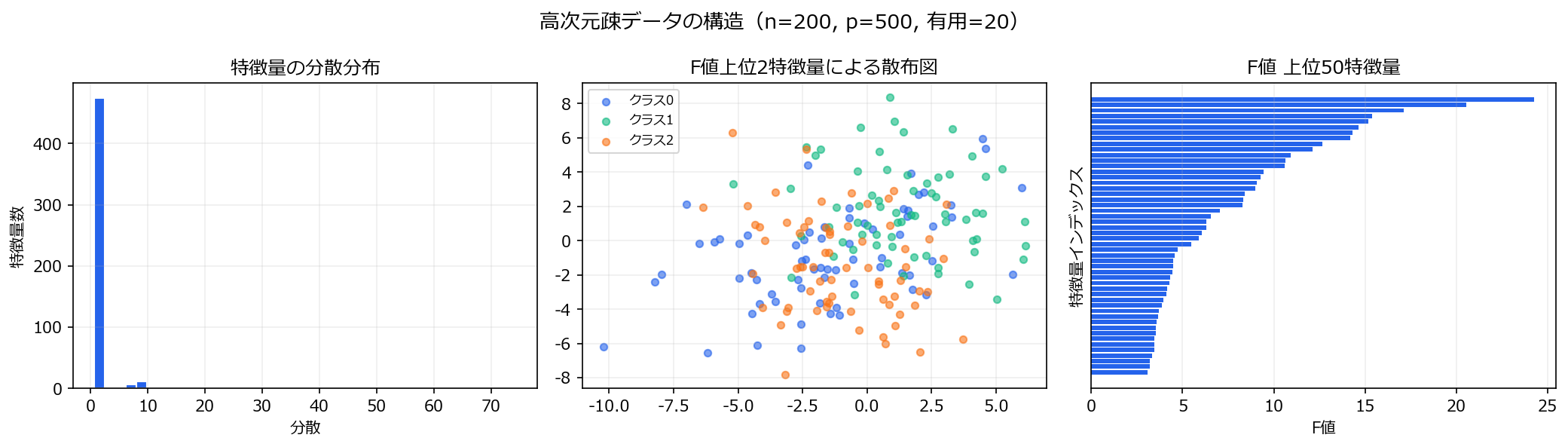
1. データの特徴 #

n=200 サンプル、p=500 特徴量の 3 クラス分類で、有用な特徴量は 20 個とその線形結合 5 個だけ、残り 475 個はクラスと無関係なノイズです。特徴量がサンプル数の 2.5 倍あるので、どのサンプルどうしの距離もノイズ 475 列の影響で似た値になり、k-NN や RBF カーネルのような距離ベースの手法は「近い点」を正しく見つけられません（次元の呪い）。

2. 合成データの生成 #

次のコードは make_classification で 200 × 500 のデータを作り、特徴量の分散のヒストグラム、F 値上位 2 特徴量の散布図、F 値上位 50 特徴量の棒グラフの 3 枚で「有用な列がどれだけ少ないか」を見ます。

 1
 2
 3
 4
 5
 6
 7
 8
 9
10
11
12
13
14
15
16
17
18
19
20
21
22
23
24
25
26
27
28
29
30
31
32
33
34
35
36
37
38
39
40
41
42
43
44
45
46
import numpy as np
import pandas as pd
import matplotlib.pyplot as plt
from sklearn.datasets import make_classification

X, y = make_classification(
    n_samples=200, n_features=500, n_informative=20,
    n_redundant=5, n_classes=3, n_clusters_per_class=1,
    random_state=42, class_sep=1.0,
)

fig, axes = plt.subplots(1, 3, figsize=(14, 4))

# 特徴量の分散分布
variances = X.var(axis=0)
axes[0].hist(variances, bins=40, color="#2563eb", edgecolor="white")
axes[0].set_title("特徴量の分散分布")
axes[0].set_xlabel("分散")
axes[0].set_ylabel("特徴量数")
axes[0].grid(alpha=0.2)

# 上位2特徴量で散布図
from sklearn.feature_selection import f_classif
f_scores, _ = f_classif(X, y)
top2 = np.argsort(f_scores)[-2:]
colors_map = {0: "#2563eb", 1: "#10b981", 2: "#f97316"}
for c in np.unique(y):
    mask = y == c
    axes[1].scatter(X[mask, top2[0]], X[mask, top2[1]], c=colors_map[c],
                    label=f"クラス{c}", alpha=0.6, s=20)
axes[1].set_title("F値上位2特徴量による散布図")
axes[1].legend(fontsize=8)
axes[1].grid(alpha=0.2)

# F値の上位50
top50_idx = np.argsort(f_scores)[-50:]
axes[2].barh(range(50), f_scores[top50_idx], color="#2563eb", height=0.8)
axes[2].set_title("F値 上位50特徴量")
axes[2].set_xlabel("F値")
axes[2].set_ylabel("特徴量インデックス")
axes[2].set_yticks([])
axes[2].grid(alpha=0.2, axis="x")

fig.suptitle("高次元疎データの構造（n=200, p=500, 有用=20）", fontsize=13)
fig.tight_layout()
plt.show()

コードの解説番号をクリックすると、コード内の該当行がハイライトされます。

6-10 行目有用 20 列 + ノイズ 480 列のデータを作る
n_informative=20 でクラスを分ける情報を持つ列を 20 個、n_redundant=5 でそれらの線形結合を 5 個作り、残り 475 個は純粋なノイズです。class_sep=1.0 は塊の離れ具合で、1.0 は「有用な列だけ見ればほぼ分けられるが、ノイズに埋もれると難しい」程度です。n_samples=200 に対して n_features=500 という比率が、このページの主題である \(p \gg n\) の状況を作っています。
15-20 行目分散だけでは有用な列を見分けられない
全 500 列の分散をヒストグラムにします。make_classification はノイズ列も有用列も標準正規分布から作るので、分散はどれも 1 前後に集まり、分散の大きさで有用な列を選ぶ VarianceThreshold がこのデータではあまり効かないことが、この 1 枚から予想できます。
23-33 行目F 値で選んだ 2 列だけなら 3 クラスは見える
f_classif は各列について「クラス間の平均差 ÷ クラス内のばらつき」の F 値を返し、np.argsort(f_scores)[-2:] で上位 2 列を取り出します。この 2 列の散布図で 3 クラスが塊として見えるなら、情報は確かに存在し、問題は 480 列のノイズに埋もれていることだけだと分かります。後の SelectKBest(f_classif, k=50) はこの F 値の上位 50 列を残す処理です。
36-42 行目F 値上位 50 列の崖を見る
F 値を大きい順に並べて 50 本の棒にすると、上位 20〜25 本が高く、その先で急に低くなる崖が見えるはずです。崖の位置が「有用な列の数」の見積もりで、SelectKBest の k を 50 にしているのは、崖より少し余裕を持たせた値です。k を 10 にすると有用列を取りこぼし、200 にするとノイズが戻ってきます。

高次元疎データの構造

3. 比較するパイプライン #

前処理	分類器
なし	Logistic(L1), Logistic(L2), SVM(linear), SVM(RBF), NaiveBayes, RandomForest
VarianceThreshold (中央値以上)	同上
SelectKBest (k=50)	同上
PCA (n=50)	同上

合計: 4前処理 × 6分類器 = 24パイプライン

4. 実験と結果 #

次のコードは 24 本のパイプラインを同じ 5 分割で交差検証し、F1-macro の平均を 4 行 × 6 列のヒートマップに並べます。すべてのパイプラインの先頭に StandardScaler を置き、前処理は交差検証の各分割の中で学習データだけから当てはめます。

 1
 2
 3
 4
 5
 6
 7
 8
 9
10
11
12
13
14
15
16
17
18
19
20
21
22
23
24
25
26
27
28
29
30
31
32
33
34
35
36
37
38
39
40
41
42
43
44
45
46
47
48
49
50
51
52
53
54
55
56
57
58
from sklearn.model_selection import cross_val_score, StratifiedKFold
from sklearn.preprocessing import StandardScaler
from sklearn.pipeline import Pipeline
from sklearn.feature_selection import VarianceThreshold, SelectKBest, f_classif
from sklearn.decomposition import PCA
from sklearn.linear_model import LogisticRegression
from sklearn.svm import SVC
from sklearn.naive_bayes import GaussianNB
from sklearn.ensemble import RandomForestClassifier
import seaborn as sns

cv = StratifiedKFold(n_splits=5, shuffle=True, random_state=42)

preprocessors = {
    "なし": None,
    "VarThresh": VarianceThreshold(threshold=np.median(X.var(axis=0))),
    "KBest50": SelectKBest(f_classif, k=50),
    "PCA50": PCA(n_components=50),
}
classifiers = {
    "Logistic(L1)": LogisticRegression(penalty="l1", solver="saga", max_iter=5000, C=1.0, random_state=42),
    "Logistic(L2)": LogisticRegression(penalty="l2", max_iter=5000, C=1.0, random_state=42),
    "SVM(linear)": SVC(kernel="linear", C=1.0, random_state=42),
    "SVM(RBF)": SVC(kernel="rbf", C=1.0, random_state=42),
    "NaiveBayes": GaussianNB(),
    "RandomForest": RandomForestClassifier(n_estimators=100, random_state=42),
}

results = []
for prep_name, prep in preprocessors.items():
    for clf_name, clf in classifiers.items():
        steps = [("scaler", StandardScaler())]
        if prep is not None:
            steps.append(("prep", prep))
        steps.append(("clf", clf))
        pipe = Pipeline(steps)
        scores = cross_val_score(pipe, X, y, cv=cv, scoring="f1_macro")
        results.append({
            "前処理": prep_name, "分類器": clf_name,
            "F1-macro": scores.mean(), "std": scores.std(),
        })

df = pd.DataFrame(results)
pivot = df.pivot_table(index="前処理", columns="分類器", values="F1-macro")
prep_order = ["なし", "VarThresh", "KBest50", "PCA50"]
clf_order = ["Logistic(L1)", "Logistic(L2)", "SVM(linear)", "SVM(RBF)", "NaiveBayes", "RandomForest"]
pivot = pivot.reindex(index=[p for p in prep_order if p in pivot.index],
                      columns=[c for c in clf_order if c in pivot.columns])

fig, ax = plt.subplots(figsize=(12, 4))
sns.heatmap(pivot, annot=True, fmt=".3f", cmap="RdYlGn",
            linewidths=0.5, ax=ax, vmin=0.3, vmax=1.0,
            cbar_kws={"label": "F1-macro（高いほど良い）"})
ax.set_title("高次元疎データ: 前処理 × 分類器 F1-macro ヒートマップ")
ax.set_xlabel("")
ax.set_ylabel("")
fig.tight_layout()
plt.show()

コードの解説番号をクリックすると、コード内の該当行がハイライトされます。

12 行目分割を固定して 24 本を同じ条件で比べる
StratifiedKFold(n_splits=5, shuffle=True, random_state=42) を 1 つ作って全パイプラインに渡すので、どの組み合わせも同じ 5 通りの学習・評価分割で採点されます。これを省いて cv=5 と書くと分割は同じになりますが、shuffle=True がなく、データの並び順に偏りがあると評価が歪みます。Stratified は 3 クラスの比率を各分割で保つ指定です。
14-19 行目4 つの前処理は「列を減らす」方法が違う
VarianceThreshold は分散が中央値以下の列を落とす（ラベルを見ない）、SelectKBest(f_classif, k=50) は F 値上位 50 列を残す（ラベルを見る）、PCA(n_components=50) は 500 列を分散最大の 50 方向に合成する（ラベルを見ない）処理です。None は前処理なしの基準で、ここが最も低ければ「前処理が効いた」と言えます。
20-27 行目6 つの分類器の中で L1 だけが自前で特徴選択をする
LogisticRegression(penalty="l1", solver="saga") は不要な係数を厳密に 0 にするので、前処理なしでも 475 列のノイズを自分で切り捨てます。penalty="l2" は係数を縮めるだけで 0 にはしません。SVC(kernel="rbf") は 500 次元の距離に依存し、GaussianNB は列ごとに独立に平均・分散を見るので高次元の影響を受けにくい、という性質の違いが結果の差になります。
30-41 行目前処理は Pipeline の中に入れてリークを防ぐ
Pipeline([("scaler", ...), ("prep", ...), ("clf", ...)]) にまとめて cross_val_score に渡すので、SelectKBest の F 値計算も PCA の軸も各分割の学習データだけから求まります。先に全 200 件で SelectKBest を当ててから交差検証すると、評価データのラベルを使って列を選んだことになり、F1 が 0.05〜0.1 ほど楽観的に出ます。scoring="f1_macro" は 3 クラスの F1 を単純平均した指標です。
43-58 行目4 × 6 の表にして色で読む
pivot_table で前処理を行、分類器を列にした表を作り、reindex で表の並びを固定してから sns.heatmap に渡します。vmin=0.3, vmax=1.0 で色の範囲を固定しているので、別のデータで再実行しても色の意味（緑なら 0.9 前後）が変わりません。annot=True, fmt=".3f" で各セルに小数 3 桁の F1-macro を書き込みます。

F1-macro ヒートマップ

読み方のポイント #

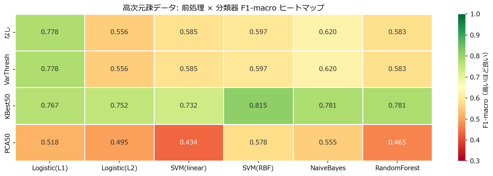
SelectKBest(k=50) や PCA(n=50) で 500 列を 50 列に絞ると、ほぼすべての分類器で F1-macro が改善します。L1 正則化の LogisticRegression は前処理なしでも比較的健闘しますが、これは内部でスパースな特徴選択を行い、475 本のノイズ列の係数を 0 にしているためです。RBF カーネルの SVM は前処理なしだと F1 が大幅に低下します。500 次元空間ではすべてのサンプル間距離がほぼ等しくなり、RBF カーネルの距離計算が機能しないからです。GaussianNB は前処理によらず安定しており、特徴量を独立に扱う仮定が、クラスと無関係なノイズ列の影響を打ち消す方向に働いています。

5. 誤差パターン分析 #

ヒートマップの最良と最悪に近い 3 つの組み合わせを、同じ 70/30 分割で学習・評価し、混同行列で「どのクラスをどのクラスと間違えたか」を比べます。

 1
 2
 3
 4
 5
 6
 7
 8
 9
10
11
12
13
14
15
16
17
18
19
20
21
22
23
24
25
26
27
from sklearn.metrics import confusion_matrix, ConfusionMatrixDisplay

# ベスト vs ワーストを固定データ分割で比較
from sklearn.model_selection import train_test_split
X_tr, X_te, y_tr, y_te = train_test_split(X, y, test_size=0.3, random_state=42, stratify=y)

configs = [
    ("KBest50 + Logistic(L1)", [("scaler", StandardScaler()), ("prep", SelectKBest(f_classif, k=50)),
                                  ("clf", LogisticRegression(penalty="l1", solver="saga", max_iter=5000, random_state=42))]),
    ("なし + SVM(RBF)", [("scaler", StandardScaler()),
                          ("clf", SVC(kernel="rbf", random_state=42))]),
    ("PCA50 + RandomForest", [("scaler", StandardScaler()), ("prep", PCA(n_components=50)),
                                ("clf", RandomForestClassifier(n_estimators=100, random_state=42))]),
]

fig, axes = plt.subplots(1, 3, figsize=(14, 4))
for i, (name, steps) in enumerate(configs):
    pipe = Pipeline(steps)
    pipe.fit(X_tr, y_tr)
    y_pred = pipe.predict(X_te)
    cm = confusion_matrix(y_te, y_pred)
    ConfusionMatrixDisplay(cm, display_labels=[0, 1, 2]).plot(ax=axes[i], cmap="Blues", colorbar=False)
    axes[i].set_title(name, fontsize=10)

fig.suptitle("混同行列の比較（テストデータ）", fontsize=13)
fig.tight_layout()
plt.show()

コードの解説番号をクリックすると、コード内の該当行がハイライトされます。

4-5 行目混同行列は 1 回の固定分割で描く
train_test_split(test_size=0.3, stratify=y) で 140 件を学習、60 件を評価に分けます。交差検証では 5 つの混同行列ができて見比べにくいので、ここでは 1 回の分割に固定し、stratify=y で 3 クラスの比率を評価側にも保ちます。60 件なので 1 セルの差 1 は約 1.7 % に当たります。
7-14 行目良い組・悪い組・中間の組を 1 つずつ選ぶ
KBest50 + Logistic(L1) はヒートマップで上位、なし + SVM(RBF) は下位、PCA50 + RandomForest は中間の代表です。3 つを同じ Pipeline の形で書いているので、違いは前処理と分類器だけです。別の組を見たいときは、このリストにタプルを 1 つ足せば 4 枚目が描かれます。
17-23 行目対角線以外の数字が誤分類
confusion_matrix の行が正解、列が予測で、対角線のセルが正解数、それ以外が「行のクラスを列のクラスと間違えた数」です。ConfusionMatrixDisplay が 3 × 3 の表を色付きで描くので、どのクラスの組が混ざりやすいかが一目で分かります。colorbar=False は 3 枚並べたときの幅を揃えるための指定です。

混同行列の比較

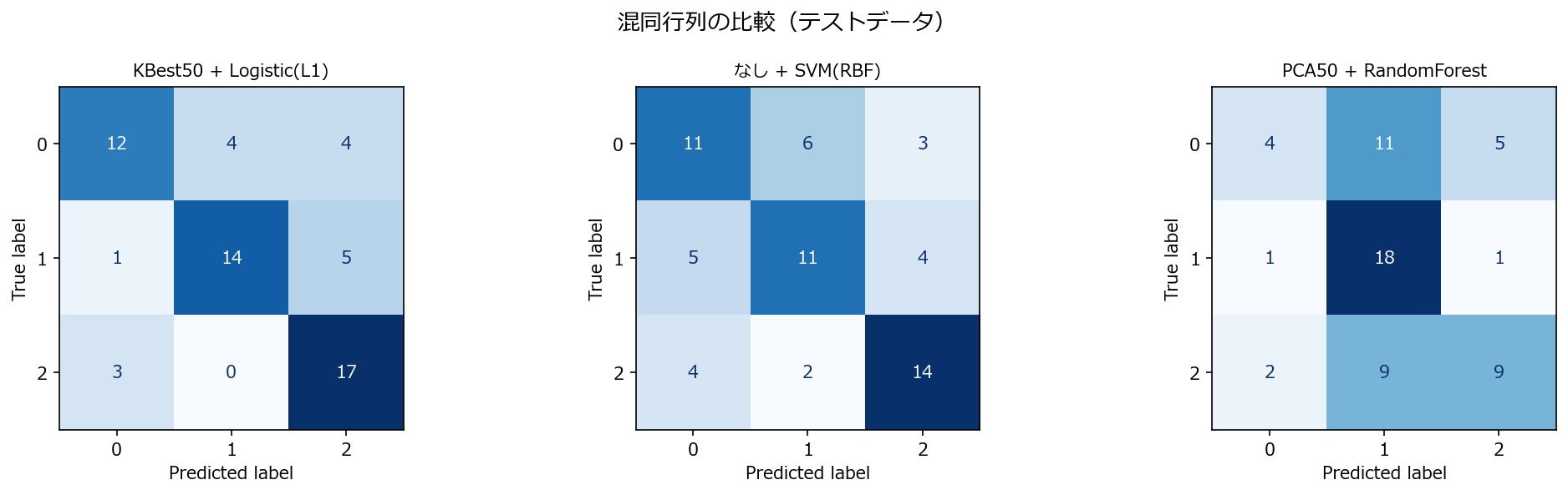
前処理なしの RBF-SVM はオフダイアゴナル（誤分類）が多く、特にクラス間の混同が激しい。KBest + L1 Logistic は対角成分が支配的で、3 クラスとも安定して分類できている。

6. よくある失敗パターン #

最初の失敗は、前処理なしで RBF カーネルを使うことです。500 次元の空間ではすべてのサンプル間距離がほぼ等しくなり、カーネルが効きません。線形カーネルを使うか、SelectKBest や PCA で次元削減を先に行います。二つ目は、全特徴量でランダムフォレストを使うことです。動きはしますが、475 個のノイズ列がスプリット候補に入るため精度が落ちます。max_features を小さく設定するか、事前に特徴選択をしてください。

まとめ #

サンプル 200 件・特徴量 500 個のデータでは、分類器の選択より「500 列を 50 列に絞る前処理」のほうが F1-macro を大きく動かしました。SelectKBest(k=50) と PCA(n_components=50) はほぼ全モデルを改善し、L1 正則化の LogisticRegression は前処理なしでも自前の特徴選択で持ちこたえます。RBF カーネルの SVM は距離が均一化する高次元で最も崩れ、GaussianNB は独立仮定のおかげで最も安定しました。特徴選択は必ず Pipeline に入れて交差検証の中で行い、評価データのラベルを使ったリークを防いでください。

ロジスティック回帰 — L1/L2正則化の基礎
SVM — カーネル法と高次元空間
ナイーブベイズ — 高次元で安定する生成モデル
F1スコア — 多クラス分類の精度指標