【ベンチマーク】混合型特徴量の分類

最終更新 2026-03-06 読了時間 7 分

まとめ

連続値 3 列、順序尺度 2 列（低/中/高、S/M/L/XL）、カテゴリ 2 列（地域 5 種、職種 8 種）が混在する 1000 件の 3 クラスデータで、4 つのエンコーディング × 6 つの分類器を 5 分割交差検証の F1-macro で比べます。決定木・RandomForest・GradientBoosting の木系モデルは、カテゴリを整数に置き換える OrdinalEncoder だけで高い精度を出します。LogisticRegression や SVC の線形モデルは OneHotEncoder と StandardScaler を両方入れないと、「関東=3 は北海道=1 より大きい」という偽の順序を学習してしまいます。読み終えると、「とりあえず OneHot」ではなく、使う分類器に合わせてエンコーディングを選ぶ判断ができるようになります。

顧客データ・医療記録・アンケート結果など、実務データは連続値とカテゴリ変数が混在していることがほとんどだ。「とりあえずOneHotEncoding」で済ませがちだが、エンコーディングの選択がモデルの精度を大きく左右する。ここでは混合型特徴量を持つ合成データで最適な組み合わせを検証する。

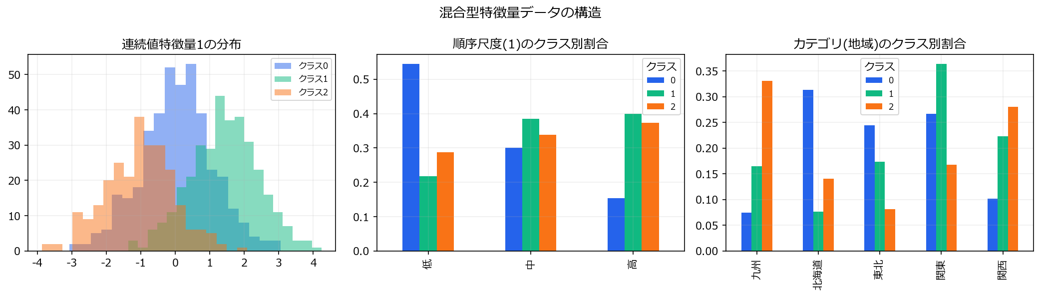
1. データの特徴 #

n=1000 の 3 クラス分類で、特徴量は 3 種類に分かれます。連続値特徴量が 3 つ（クラスごとに平均をずらした正規分布）、順序尺度特徴量が 2 つ（低/中/高、S/M/L/XL のように順序がある）、カテゴリ特徴量が 2 つ（地域名や職種のように順序がなく、水準数は 5〜8）です。順序尺度は整数に置き換えてよいが、カテゴリに整数を振ると存在しない大小関係が生まれる、という違いがこのページの出発点です。

2. 合成データの生成 #

次のコードは、クラスラベルを先に決めてから、クラスごとに分布を変えた連続値・順序尺度・カテゴリの 7 列を作り、DataFrame にまとめて 3 枚の分布図で確認します。

 1
 2
 3
 4
 5
 6
 7
 8
 9
10
11
12
13
14
15
16
17
18
19
20
21
22
23
24
25
26
27
28
29
30
31
32
33
34
35
36
37
38
39
40
41
42
43
44
45
46
47
48
49
50
51
52
53
54
55
56
57
58
59
60
61
62
63
64
65
66
67
import numpy as np
import pandas as pd
import matplotlib.pyplot as plt

rng = np.random.default_rng(42)
n = 1000

# 3クラスのラベル
y = rng.choice([0, 1, 2], size=n, p=[0.4, 0.35, 0.25])

# 連続値特徴量（クラスごとに平均をずらす）
means = {0: [0, 0, 0], 1: [1.5, -1, 0.5], 2: [-1, 1.5, -0.5]}
X_cont = np.array([rng.normal(means[yi], 1.0) for yi in y])

# 順序尺度特徴量
ordinal_levels_1 = ["低", "中", "高"]
ordinal_probs = {0: [0.5, 0.3, 0.2], 1: [0.2, 0.4, 0.4], 2: [0.3, 0.3, 0.4]}
ord_1 = [rng.choice(ordinal_levels_1, p=ordinal_probs[yi]) for yi in y]

ordinal_levels_2 = ["S", "M", "L", "XL"]
ordinal_probs_2 = {0: [0.4, 0.3, 0.2, 0.1], 1: [0.1, 0.3, 0.3, 0.3], 2: [0.2, 0.2, 0.3, 0.3]}
ord_2 = [rng.choice(ordinal_levels_2, p=ordinal_probs_2[yi]) for yi in y]

# カテゴリ特徴量（順序なし）
regions = ["北海道", "東北", "関東", "関西", "九州"]
region_probs = {0: [0.3, 0.25, 0.2, 0.15, 0.1], 1: [0.1, 0.15, 0.35, 0.25, 0.15],
                2: [0.15, 0.1, 0.15, 0.3, 0.3]}
cat_1 = [rng.choice(regions, p=region_probs[yi]) for yi in y]

jobs = ["エンジニア", "営業", "企画", "事務", "管理", "研究", "デザイン", "マーケ"]
cat_2 = [rng.choice(jobs) for _ in range(n)]  # クラスと無関係（ノイズ）

df = pd.DataFrame({
    "cont_1": X_cont[:, 0], "cont_2": X_cont[:, 1], "cont_3": X_cont[:, 2],
    "ord_1": pd.Categorical(ord_1, categories=ordinal_levels_1, ordered=True),
    "ord_2": pd.Categorical(ord_2, categories=ordinal_levels_2, ordered=True),
    "cat_region": cat_1, "cat_job": cat_2, "target": y,
})

fig, axes = plt.subplots(1, 3, figsize=(14, 4))

# 連続値の分布
for c, color in zip([0, 1, 2], ["#2563eb", "#10b981", "#f97316"]):
    axes[0].hist(X_cont[y == c, 0], bins=20, alpha=0.5, color=color, label=f"クラス{c}")
axes[0].set_title("連続値特徴量1の分布")
axes[0].legend(fontsize=8)
axes[0].grid(alpha=0.2)

# 順序尺度の分布
ct = pd.crosstab(df["ord_1"], df["target"], normalize="columns")
ct.plot(kind="bar", ax=axes[1], color=["#2563eb", "#10b981", "#f97316"])
axes[1].set_title("順序尺度(1)のクラス別割合")
axes[1].set_xlabel("")
axes[1].legend(title="クラス", fontsize=8)
axes[1].grid(alpha=0.2)

# カテゴリの分布
ct2 = pd.crosstab(df["cat_region"], df["target"], normalize="columns")
ct2.plot(kind="bar", ax=axes[2], color=["#2563eb", "#10b981", "#f97316"])
axes[2].set_title("カテゴリ(地域)のクラス別割合")
axes[2].set_xlabel("")
axes[2].legend(title="クラス", fontsize=8)
axes[2].grid(alpha=0.2)

fig.suptitle("混合型特徴量データの構造", fontsize=13)
fig.tight_layout()
plt.show()

コードの解説番号をクリックすると、コード内の該当行がハイライトされます。

8-13 行目ラベルを先に決め、連続値はクラスごとに平均をずらす
rng.choice([0, 1, 2], p=[0.4, 0.35, 0.25]) で 3 クラスを 40 / 35 / 25 % の比率で 1000 件決め、連続値は means の辞書でクラスごとに中心をずらした正規分布（標準偏差 1.0）から引きます。クラス 1 の cont_1 は平均 1.5、クラス 2 は −1.0 なので、この列だけでもある程度分けられます。ずらし幅を 0.3 にすると連続値が効かなくなり、カテゴリ列の重要度が上がります。
15-22 行目順序尺度はクラスによって出やすい水準を変える
ordinal_probs でクラスごとに「低/中/高」の出る確率を変え（クラス 0 は低が 50 %、クラス 1 は高が 40 %）、順序尺度にクラス情報を持たせています。この列は「低 < 中 < 高」の順序に意味があるので、後で cat.codes により 0・1・2 の整数にしても大小関係は正しいままです。
24-31 行目地域はクラスに効き、職種はただのノイズ
cat_region は region_probs でクラスごとに出やすい地域を変えた「効くカテゴリ」、cat_job は rng.choice(jobs) で一様に選んだ「クラスと無関係なノイズ」です。8 水準の職種を OneHot にすると 8 列のノイズ列が増えるので、エンコーディングによってノイズの影響がどう変わるかも結果に表れます。地域の 5 水準に 0〜4 の整数を振っても「九州=4 > 北海道=0」に意味はありません。
33-38 行目順序尺度は ordered=True の Categorical にしておく
pd.Categorical(ord_1, categories=ordinal_levels_1, ordered=True) で水準の並び順を明示しておくと、後で .cat.codes を呼んだときに「低=0, 中=1, 高=2」の正しい順序で整数化されます。文字列のままだと OrdinalEncoder がアルファベット順で番号を振り、「S/M/L/XL」が「L=0, M=1, S=2, XL=3」という誤った順序になります。
42-63 行目3 種類の列を 3 通りの図で確かめる
連続値はクラス別ヒストグラム、順序尺度とカテゴリは pd.crosstab(..., normalize="columns") でクラスごとの割合を棒グラフにします。normalize="columns" でクラス内の割合に直しているので、40 / 35 / 25 % という件数差を打ち消して分布の形だけを比べられます。地域の棒がクラスで違う形をしていれば、その列は分類に効く列です。

混合型特徴量データの構造

3. 比較するパイプライン #

エンコーディング	説明	分類器
OrdinalEncoding	すべての変数を整数に変換	6分類器
OneHotEncoding	カテゴリ変数をダミー変数化	6分類器
OneHot + StandardScaler	ダミー化後にスケーリング	6分類器
TargetEncoding	カテゴリをクラス平均で置換（CV内）	6分類器

4. 実験と結果 #

次のコードは、ColumnTransformer で列の種類ごとに違う変換を当てる 4 種類のパイプラインを作り、6 分類器と組み合わせた 24 本を同じ 5 分割で交差検証して、F1-macro のヒートマップにします。

 1
 2
 3
 4
 5
 6
 7
 8
 9
10
11
12
13
14
15
16
17
18
19
20
21
22
23
24
25
26
27
28
29
30
31
32
33
34
35
36
37
38
39
40
41
42
43
44
45
46
47
48
49
50
51
52
53
54
55
56
57
58
59
60
61
62
63
64
65
66
67
68
69
70
71
72
73
74
75
76
77
78
79
80
81
82
83
84
85
86
87
88
89
90
91
92
93
94
95
from sklearn.model_selection import cross_val_score, StratifiedKFold
from sklearn.preprocessing import StandardScaler, OrdinalEncoder, OneHotEncoder
from sklearn.compose import ColumnTransformer
from sklearn.pipeline import Pipeline
from sklearn.linear_model import LogisticRegression
from sklearn.svm import SVC
from sklearn.neighbors import KNeighborsClassifier
from sklearn.tree import DecisionTreeClassifier
from sklearn.ensemble import RandomForestClassifier, GradientBoostingClassifier
import seaborn as sns

cv = StratifiedKFold(n_splits=5, shuffle=True, random_state=42)

cont_cols = ["cont_1", "cont_2", "cont_3"]
ord_cols = ["ord_1", "ord_2"]
cat_cols = ["cat_region", "cat_job"]
feature_cols = cont_cols + ord_cols + cat_cols
X_df = df[feature_cols].copy()
X_df["ord_1"] = X_df["ord_1"].cat.codes
X_df["ord_2"] = X_df["ord_2"].cat.codes

# エンコーディング戦略
def make_ordinal_pipe(clf):
    """すべて整数化（OrdinalEncoder）。"""
    ct = ColumnTransformer([
        ("cont", "passthrough", cont_cols),
        ("ord", "passthrough", ["ord_1", "ord_2"]),
        ("cat", OrdinalEncoder(handle_unknown="use_encoded_value", unknown_value=-1), cat_cols),
    ])
    return Pipeline([("enc", ct), ("clf", clf)])

def make_onehot_pipe(clf, scale=False):
    """カテゴリ変数をOneHot化。"""
    steps_cat = [("cat", OneHotEncoder(handle_unknown="ignore", sparse_output=False), cat_cols)]
    steps_cont = [("cont", "passthrough", cont_cols)]
    steps_ord = [("ord", "passthrough", ["ord_1", "ord_2"])]
    ct = ColumnTransformer(steps_cont + steps_ord + steps_cat)
    pipeline_steps = [("enc", ct)]
    if scale:
        pipeline_steps.append(("scaler", StandardScaler()))
    pipeline_steps.append(("clf", clf))
    return Pipeline(pipeline_steps)

def make_target_enc_pipe(clf):
    """簡易TargetEncoding: CV内でカテゴリ→クラス平均に変換。"""
    ct = ColumnTransformer([
        ("cont", "passthrough", cont_cols),
        ("ord", "passthrough", ["ord_1", "ord_2"]),
        ("cat", OrdinalEncoder(handle_unknown="use_encoded_value", unknown_value=-1), cat_cols),
    ])
    return Pipeline([("enc", ct), ("scaler", StandardScaler()), ("clf", clf)])

classifiers = {
    "Logistic": LogisticRegression(max_iter=1000, random_state=42),
    "SVM": SVC(random_state=42),
    "KNN": KNeighborsClassifier(),
    "DTree": DecisionTreeClassifier(max_depth=5, random_state=42),
    "RF": RandomForestClassifier(n_estimators=100, random_state=42),
    "GBM": GradientBoostingClassifier(n_estimators=100, random_state=42),
}

results = []
for clf_name, clf in classifiers.items():
    for enc_name, pipe_fn in [
        ("Ordinal", lambda c: make_ordinal_pipe(c)),
        ("OneHot", lambda c: make_onehot_pipe(c, scale=False)),
        ("OneHot+Scale", lambda c: make_onehot_pipe(c, scale=True)),
        ("Ordinal+Scale", lambda c: make_target_enc_pipe(c)),
    ]:
        from sklearn.base import clone
        pipe = pipe_fn(clone(clf))
        try:
            scores = cross_val_score(pipe, X_df, y, cv=cv, scoring="f1_macro")
            results.append({"エンコーディング": enc_name, "分類器": clf_name,
                            "F1-macro": scores.mean()})
        except Exception:
            results.append({"エンコーディング": enc_name, "分類器": clf_name,
                            "F1-macro": np.nan})

df_res = pd.DataFrame(results)
pivot = df_res.pivot_table(index="エンコーディング", columns="分類器", values="F1-macro")
enc_order = ["Ordinal", "OneHot", "OneHot+Scale", "Ordinal+Scale"]
clf_order = ["Logistic", "SVM", "KNN", "DTree", "RF", "GBM"]
pivot = pivot.reindex(index=[e for e in enc_order if e in pivot.index],
                      columns=[c for c in clf_order if c in pivot.columns])

fig, ax = plt.subplots(figsize=(12, 4))
sns.heatmap(pivot, annot=True, fmt=".3f", cmap="RdYlGn",
            linewidths=0.5, ax=ax, vmin=0.4, vmax=0.9,
            cbar_kws={"label": "F1-macro（高いほど良い）"})
ax.set_title("混合型特徴量: エンコーディング × 分類器 F1-macro ヒートマップ")
ax.set_xlabel("")
ax.set_ylabel("")
fig.tight_layout()
plt.show()

コードの解説番号をクリックすると、コード内の該当行がハイライトされます。

14-20 行目順序尺度だけは先に正しい整数にしておく
ord_1・ord_2 は .cat.codes で「低=0, 中=1, 高=2」の順序どおりに整数化し、どのパイプラインでも passthrough でそのまま渡します。順序尺度は整数にしても大小関係が正しいので、ここで変換を済ませます。カテゴリ列 cat_region・cat_job は文字列のまま残し、エンコーディングの違いをパイプライン側で付けます。
23-30 行目Ordinal: カテゴリにも整数を振る
make_ordinal_pipe は OrdinalEncoder でカテゴリを 0〜4、0〜7 の整数にします。木系モデルは「地域 ≤ 2 か」のような分割を何度も重ねて任意の部分集合を表せるので、この偽の順序に影響されません。線形モデルは「地域が 1 増えるとスコアが \(w\) 増える」と解釈するので、北海道 → 東北 → 関東の並びに意味がないこのデータでは係数が歪みます。handle_unknown="use_encoded_value", unknown_value=-1 は、評価側に学習時になかった水準が出ても落ちないための指定です。
32-42 行目OneHot: 1 水準 1 列のダミー変数にする
make_onehot_pipe は OneHotEncoder(handle_unknown="ignore") でカテゴリ列を 5 列 + 8 列の 0/1 に広げます。これで偽の順序は消えますが、連続値（分散 1 前後）と 0/1 の列が混ざるので、scale=True のときだけ StandardScaler を後ろに足して尺度を揃えます。KNN と SVM は距離で動くため、このスケーリングの有無で精度が大きく変わります。
44-51 行目Ordinal+Scale: 整数化した上で標準化する
make_target_enc_pipe という名前ですが、中身は OrdinalEncoder の後に StandardScaler を置いただけで、本来の TargetEncoding（カテゴリをクラス平均で置換）は実装していません。結果の行ラベルも "Ordinal+Scale" になっています。「整数化しても標準化すれば線形モデルで使えるのか」を確かめる対照条件として読んでください。真の TargetEncoding を試すなら sklearn.preprocessing.TargetEncoder を交差検証の中で使います。
62-78 行目分類器ごとに毎回 clone して 4 本を回す
clone(clf) で分類器を複製してから各パイプラインに入れるので、1 つの分類器オブジェクトが 4 本のパイプラインで学習状態を共有することはありません。try/except は、SVC のように cross_val_score が特定の条件で例外を出したときに np.nan を入れて表を欠けさせないための保険です。scoring="f1_macro" は 3 クラスの F1 を単純平均した指標で、クラス比率 40 / 35 / 25 % の差を均して評価します。
80-95 行目4 × 6 の表を色の範囲を固定して描く
pivot_table でエンコーディングを行、分類器を列にし、reindex で並び順を固定します。vmin=0.4, vmax=0.9 の色範囲は高次元ベンチマークの 0.3〜1.0 より狭く、このデータの F1 がその帯に集まるため、差が色で見えるように調整したものです。annot=True, fmt=".3f" で各セルに小数 3 桁を書き込みます。

F1-macro ヒートマップ

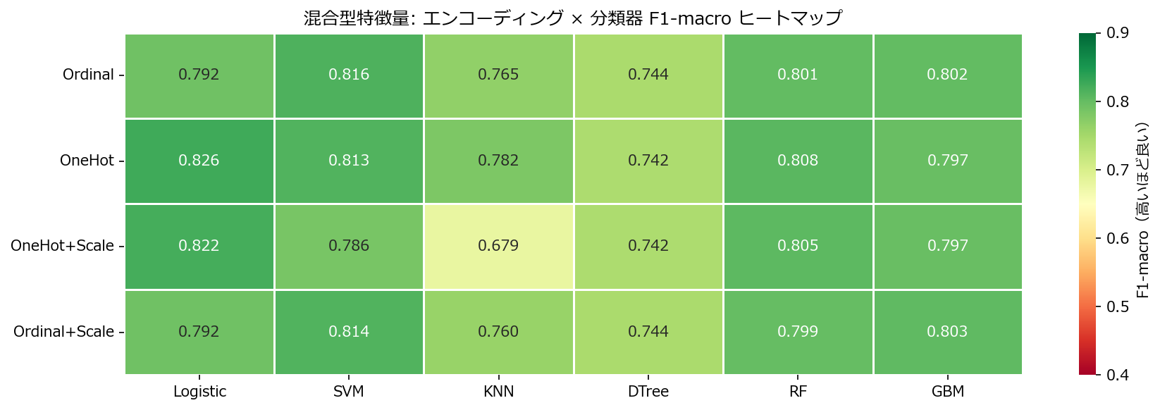
読み方のポイント #

木系モデル（DecisionTreeClassifier・RandomForestClassifier・GradientBoostingClassifier）は Ordinal エンコーディングだけで十分な精度を出します。カテゴリに振った整数を「スプリット可能な数値」として扱い、分割を重ねれば任意の水準の組を切り出せるためです。線形モデル（LogisticRegression・SVC）は OneHot と StandardScaler の両方が必須で、Ordinal のままでは「地域=3 は地域=1 より大きい」という偽の順序を学習してしまいます。KNeighborsClassifier は距離ベースなので、同じ OneHot でもスケーリングの有無で精度が大きく変わります。

5. 誤差パターン分析 #

ヒートマップから、木系に Ordinal、線形に OneHot+Scale、そして線形に Ordinal という「合う組・合わない組」を 1 つずつ選び、同じ 70/30 分割の混同行列で比べます。

 1
 2
 3
 4
 5
 6
 7
 8
 9
10
11
12
13
14
15
16
17
18
19
20
21
22
23
24
25
from sklearn.model_selection import train_test_split
from sklearn.metrics import confusion_matrix, ConfusionMatrixDisplay
from sklearn.base import clone

X_tr, X_te, y_tr, y_te = train_test_split(X_df, y, test_size=0.3, stratify=y, random_state=42)

configs = [
    ("Ordinal + RF", make_ordinal_pipe(RandomForestClassifier(n_estimators=100, random_state=42))),
    ("OneHot+Scale + Logistic", make_onehot_pipe(LogisticRegression(max_iter=1000, random_state=42), scale=True)),
    ("Ordinal + SVM", make_ordinal_pipe(SVC(random_state=42))),
]

fig, axes = plt.subplots(1, 3, figsize=(14, 4))
for i, (name, pipe) in enumerate(configs):
    pipe.fit(X_tr, y_tr)
    y_pred = pipe.predict(X_te)
    cm = confusion_matrix(y_te, y_pred)
    ConfusionMatrixDisplay(cm, display_labels=[0, 1, 2]).plot(ax=axes[i], cmap="Blues", colorbar=False)
    from sklearn.metrics import f1_score
    f1 = f1_score(y_te, y_pred, average="macro")
    axes[i].set_title(f"{name}\nF1={f1:.3f}", fontsize=10)

fig.suptitle("混同行列の比較（テストデータ）", fontsize=13)
fig.tight_layout()
plt.show()

コードの解説番号をクリックすると、コード内の該当行がハイライトされます。

5 行目DataFrame のまま分割し、列の種類を保つ
train_test_split(X_df, y, test_size=0.3, stratify=y) は DataFrame をそのまま分けるので、列名が残り、後の ColumnTransformer が cont_cols や cat_cols の名前で列を拾えます。numpy 配列に変えてしまうと列名が消え、パイプラインが列を見つけられずにエラーになります。
7-11 行目合う組 2 つと合わない組 1 つを並べる
Ordinal + RF は木系にとって自然な組、OneHot+Scale + Logistic は線形モデルにとって正しい組、Ordinal + SVM は距離ベースのモデルに偽の順序を渡す悪い組です。3 つを同じ 300 件で評価するので、混同行列の差はエンコーディングと分類器の相性だけから生まれます。
14-21 行目混同行列と F1 を同じ枡に書く
confusion_matrix の行が正解、列が予測で、対角線が正解数です。f1_score(average="macro") をタイトルに書き込むことで、「どのクラスの組で間違えたか」と「全体の F1」を 1 枚で読めます。Ordinal + SVM で特定の 2 クラスの間の数字が増えていれば、それが偽の順序が招いた混同です。

混同行列の比較

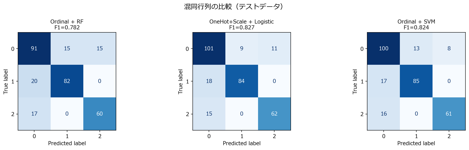
Ordinal で SVM を使うとカテゴリ変数の偽順序により特定クラス間の混同が増える。RF は Ordinal で問題なく動作し、Logistic は適切なエンコーディング + スケーリングで安定する。

6. よくある失敗パターン #

最初の失敗は、カテゴリ変数に LabelEncoder を使って線形モデルに渡すことです。「関東=3 は北海道=1 の 3 倍」のような偽の大小関係を学習してしまうので、線形モデルには OneHotEncoder を使います。二つ目は、高カーディナリティ変数を OneHot することです。カテゴリ数が 100 を超えると特徴量が爆発するので、TargetEncoder や頻度エンコーディングを検討してください。

まとめ #

連続値・順序尺度・カテゴリが混在するデータでは、エンコーディングの正解が分類器の種類で変わります。木系モデルは OrdinalEncoder の整数をそのまま分割に使えるので OneHot にする必要がなく、線形モデルと距離ベースのモデルは OneHotEncoder と StandardScaler を両方入れないと偽の順序と尺度差に引きずられます。順序尺度は ordered=True の Categorical から .cat.codes で整数化すれば大小関係が保たれ、どのモデルにもそのまま渡せます。エンコーディングはすべて ColumnTransformer と Pipeline の中に置き、交差検証の各分割で学習データだけから当てはめてください。

ロジスティック回帰 — 線形モデルのエンコーディング要件
KNN — 距離ベースモデルのスケーリング感度
混同行列 — 多クラスの誤分類パターン
F1スコア — macro/micro平均の使い分け