【ベンチマーク】ラベルノイズのある分類

 1
 2
 3
 4
 5
 6
 7
 8
 9
10
11
12
13
14
15
16
17
18
19
20
21
22
23
24
25
26
27
28
29
30
31
32
33
34
35
36
37
38
39
40
41
42
43
44
45

import numpy as np
import pandas as pd
import matplotlib.pyplot as plt
from sklearn.datasets import make_classification
from sklearn.model_selection import train_test_split

X, y_clean = make_classification(
    n_samples=1000, n_features=5, n_informative=4,
    n_redundant=1, n_classes=2, class_sep=1.5,
    random_state=42,
)
X_train, X_test, y_train_clean, y_test = train_test_split(
    X, y_clean, test_size=0.3, random_state=42, stratify=y_clean
)

# 学習データの15%をランダムに反転
rng = np.random.default_rng(42)
noise_rate = 0.15
n_flip = int(len(y_train_clean) * noise_rate)
flip_idx = rng.choice(len(y_train_clean), size=n_flip, replace=False)
y_train_noisy = y_train_clean.copy()
y_train_noisy[flip_idx] = 1 - y_train_noisy[flip_idx]

fig, axes = plt.subplots(1, 2, figsize=(12, 5))

# クリーンラベル
colors_clean = ["#2563eb" if label == 0 else "#10b981" for label in y_train_clean]
axes[0].scatter(X_train[:, 0], X_train[:, 1], c=colors_clean, alpha=0.5, s=15)
axes[0].set_title(f"クリーンラベル（学習データ, n={len(y_train_clean)}）")
axes[0].grid(alpha=0.2)

# ノイズラベル（反転箇所を強調）
colors_noisy = ["#94a3b8"] * len(y_train_noisy)
for idx in flip_idx:
    colors_noisy[idx] = "#ef4444"
axes[1].scatter(X_train[:, 0], X_train[:, 1], c=colors_noisy, alpha=0.5, s=15)
axes[1].scatter(X_train[flip_idx, 0], X_train[flip_idx, 1],
                facecolors="none", edgecolors="#ef4444", s=50, linewidths=1.5, label="反転ラベル")
axes[1].set_title(f"ノイズラベル（赤丸 = 反転, {noise_rate*100:.0f}%）")
axes[1].legend()
axes[1].grid(alpha=0.2)

fig.suptitle("ラベルノイズの可視化", fontsize=13)
fig.tight_layout()
plt.show()

 1
 2
 3
 4
 5
 6
 7
 8
 9
10
11
12
13
14
15
16
17
18
19
20
21
22
23
24
25
26
27
28
29
30
31
32
33
34
35
36
37
38
39
40
41
42
43
44
45
46
47
48
49
50
51
52
53
54
55
56
57
58
59
60
61
62
63
64

from sklearn.preprocessing import StandardScaler
from sklearn.linear_model import LogisticRegression
from sklearn.svm import SVC
from sklearn.neighbors import KNeighborsClassifier
from sklearn.ensemble import RandomForestClassifier, GradientBoostingClassifier
from sklearn.metrics import accuracy_score
from sklearn.model_selection import cross_val_predict
import seaborn as sns

scaler = StandardScaler()
X_tr_s = scaler.fit_transform(X_train)
X_te_s = scaler.transform(X_test)

# --- ラベルクリーニング ---
# 交差検証で予測確率を取得し、確信度が低いサンプルを除去
lr_cv = LogisticRegression(max_iter=1000, random_state=42)
proba = cross_val_predict(lr_cv, X_tr_s, y_train_noisy, cv=5, method="predict_proba")
predicted_label = proba.argmax(axis=1)
confidence = proba.max(axis=1)

# 「予測と実ラベルが異なり、かつ確信度が高い」サンプルを除去
suspect = (predicted_label != y_train_noisy) & (confidence > 0.7)
clean_mask = ~suspect
X_tr_cleaned = X_tr_s[clean_mask]
y_tr_cleaned = y_train_noisy[clean_mask]

classifiers = {
    "Logistic": LogisticRegression(max_iter=1000, random_state=42),
    "SVM(linear)": SVC(kernel="linear", random_state=42),
    "SVM(RBF)": SVC(kernel="rbf", random_state=42),
    "KNN": KNeighborsClassifier(),
    "RF": RandomForestClassifier(n_estimators=100, random_state=42),
    "GBM": GradientBoostingClassifier(n_estimators=100, random_state=42),
}

results = []
for name, clf_template in classifiers.items():
    for condition, X_fit, y_fit in [
        ("ノイズ", X_tr_s, y_train_noisy),
        ("クリーニング後", X_tr_cleaned, y_tr_cleaned),
        ("クリーン（参考）", X_tr_s, y_train_clean),
    ]:
        from sklearn.base import clone
        clf = clone(clf_template)
        clf.fit(X_fit, y_fit)
        acc = accuracy_score(y_test, clf.predict(X_te_s))
        results.append({"条件": condition, "分類器": name, "Accuracy": acc})

df = pd.DataFrame(results)
pivot = df.pivot_table(index="条件", columns="分類器", values="Accuracy")
cond_order = ["ノイズ", "クリーニング後", "クリーン（参考）"]
clf_order = ["Logistic", "SVM(linear)", "SVM(RBF)", "KNN", "RF", "GBM"]
pivot = pivot.reindex(index=[c for c in cond_order if c in pivot.index],
                      columns=[c for c in clf_order if c in pivot.columns])

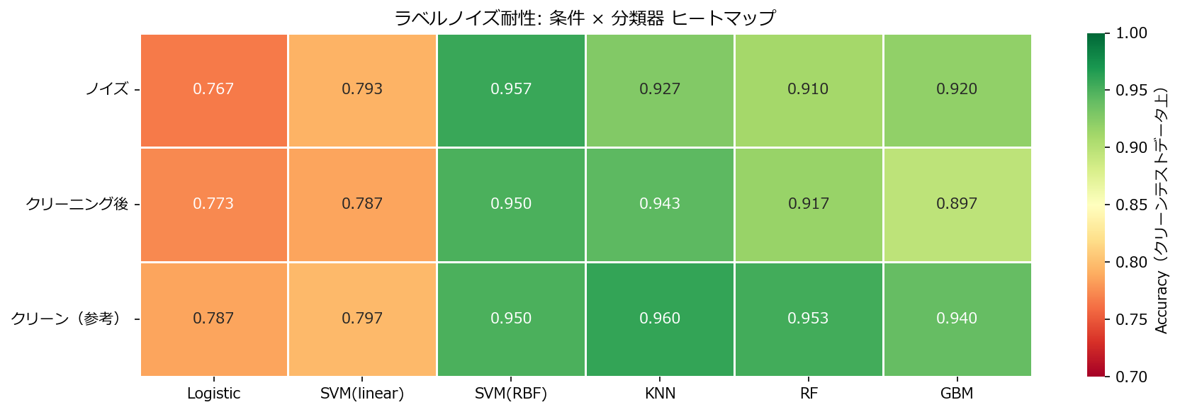
fig, ax = plt.subplots(figsize=(12, 4))
sns.heatmap(pivot, annot=True, fmt=".3f", cmap="RdYlGn",
            linewidths=0.5, ax=ax, vmin=0.7, vmax=1.0,
            cbar_kws={"label": "Accuracy（クリーンテストデータ上）"})
ax.set_title("ラベルノイズ耐性: 条件 × 分類器 ヒートマップ")
ax.set_xlabel("")
ax.set_ylabel("")
fig.tight_layout()
plt.show()

 1
 2
 3
 4
 5
 6
 7
 8
 9
10
11
12
13
14
15
16
17
18
19

from sklearn.metrics import confusion_matrix, ConfusionMatrixDisplay

fig, axes = plt.subplots(1, 3, figsize=(14, 4))
configs = [
    ("ノイズ + SVM(RBF)", SVC(kernel="rbf", random_state=42), X_tr_s, y_train_noisy),
    ("クリーニング + SVM(RBF)", SVC(kernel="rbf", random_state=42), X_tr_cleaned, y_tr_cleaned),
    ("クリーン + SVM(RBF)", SVC(kernel="rbf", random_state=42), X_tr_s, y_train_clean),
]
for i, (name, clf, X_fit, y_fit) in enumerate(configs):
    clf.fit(X_fit, y_fit)
    y_pred = clf.predict(X_te_s)
    cm = confusion_matrix(y_test, y_pred)
    ConfusionMatrixDisplay(cm, display_labels=["0", "1"]).plot(ax=axes[i], cmap="Blues", colorbar=False)
    acc = accuracy_score(y_test, y_pred)
    axes[i].set_title(f"{name}\nAcc={acc:.3f}", fontsize=10)

fig.suptitle("SVM(RBF) の混同行列: ノイズの影響", fontsize=13)
fig.tight_layout()
plt.show()