線形判別分析 (LDA) | クラスを分ける方向を学ぶ

まとめ

LDA はクラス間分散とクラス内分散の比を最大化する方向を求め、分類と次元削減の両方に利用できます。
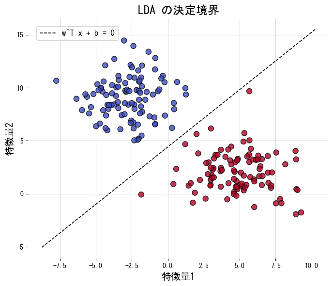
決定境界は $\mathbf{w}^\top \mathbf{x} + b = 0$ の形になり、2次元なら直線、3次元なら平面として幾何的に解釈できます。
各クラスが同一共分散を持つガウス分布だと仮定すると、ベイズ最適に近い分類器を構築できます。
scikit-learn の LinearDiscriminantAnalysis を使えば、決定境界の描画や射影後の特徴量の確認が容易です。

直感 #

LDA は「同じクラスのサンプルは近づけ、異なるクラスのサンプルは遠ざける」方向を探します。その方向に射影するとクラスが分離しやすくなり、直接分類に使ったり、低次元に圧縮して別の分類器に渡したりできます。

数式で見る #

2 クラスの場合、射影方向 $\mathbf{w}$ は

$$ J(\mathbf{w}) = \frac{\mathbf{w}^\top \mathbf{S}_B \mathbf{w}}{\mathbf{w}^\top \mathbf{S}_W \mathbf{w}} $$

を最大化することで求めます。ここで $\mathbf{S}_B$ はクラス間散布行列、$\mathbf{S}_W$ はクラス内散布行列です。多クラスでは最大でクラス数マイナス1個の射影方向が得られ、次元削減に利用できます。

Pythonによる実験 #

次のコードは2クラスの人工データに LDA を適用し、決定境界と射影後の1次元特徴量を描画します。transform を呼ぶと射影されたデータを直接取得できます。

from __future__ import annotations

import japanize_matplotlib
import matplotlib.pyplot as plt
import numpy as np
from sklearn.datasets import make_blobs
from sklearn.discriminant_analysis import LinearDiscriminantAnalysis
from sklearn.metrics import accuracy_score


def run_lda_demo(
    n_samples: int = 200,
    random_state: int = 42,
    title_boundary: str = "LDA の決定境界",
    title_projection: str = "LDA による一次元射影",
    xlabel: str = "特徴量1",
    ylabel: str = "特徴量2",
    hist_xlabel: str = "射影後の特徴量",
    class0_label: str = "クラス0",
    class1_label: str = "クラス1",
) -> dict[str, float]:
    """Train LDA on synthetic blobs and plot boundary plus projection."""
    japanize_matplotlib.japanize()
    X, y = make_blobs(
        n_samples=n_samples,
        centers=2,
        n_features=2,
        cluster_std=2.0,
        random_state=random_state,
    )

    clf = LinearDiscriminantAnalysis(store_covariance=True)
    clf.fit(X, y)

    accuracy = float(accuracy_score(y, clf.predict(X)))
    w = clf.coef_[0]
    b = float(clf.intercept_[0])

    xs = np.linspace(X[:, 0].min() - 1, X[:, 0].max() + 1, 300)
    ys_boundary = -(w[0] / w[1]) * xs - b / w[1]

    fig, ax = plt.subplots(figsize=(7, 6))
    ax.set_title(title_boundary)
    ax.scatter(X[:, 0], X[:, 1], c=y, cmap="coolwarm", edgecolor="k", alpha=0.8)
    ax.plot(xs, ys_boundary, "k--", lw=1.2, label="w^T x + b = 0")
    ax.set_xlabel(xlabel)
    ax.set_ylabel(ylabel)
    ax.legend(loc="best")
    ax.grid(alpha=0.25)
    fig.tight_layout()
    plt.show()

    X_proj = clf.transform(X)[:, 0]

    fig, ax = plt.subplots(figsize=(8, 4))
    ax.set_title(title_projection)
    ax.hist(X_proj[y == 0], bins=20, alpha=0.7, label=class0_label)
    ax.hist(X_proj[y == 1], bins=20, alpha=0.7, label=class1_label)
    ax.set_xlabel(hist_xlabel)
    ax.legend(loc="best")
    ax.grid(alpha=0.25)
    fig.tight_layout()
    plt.show()

    return {"accuracy": accuracy}


metrics = run_lda_demo(
    title_boundary="LDA の決定境界",
    title_projection="LDA による一次元射影",
    xlabel="特徴量1",
    ylabel="特徴量2",
    hist_xlabel="射影後の特徴量",
    class0_label="クラス0",
    class1_label="クラス1",
)
print(f"訓練精度: {metrics['accuracy']:.3f}")

transform を呼ぶと射影されたデータを直接取得できますの図

参考文献 #

Fisher, R. A. (1936). The Use of Multiple Measurements in Taxonomic Problems. Annals of Eugenics, 7(2), 179 E88.
Hastie, T., Tibshirani, R., & Friedman, J. (2009). The Elements of Statistical Learning. Springer.