2.2.1
ロジスティック回帰
- ロジスティック回帰は入力の線形結合をシグモイド関数に通し、クラス1に属する確率を直接推定する二値分類モデルです。
- 出力が \([0, 1]\) に収まるため、意思決定のしきい値を柔軟に調整でき、係数は対数オッズ比として解釈できます。
- 学習はクロスエントロピー損失(対数尤度の最大化)で行い、L1/L2 正則化を組み合わせると過学習を抑えられます。
- scikit-learn の
LogisticRegressionを使えば、前処理から決定境界の可視化まで数行で実装できます。
直感 #
線形回帰の出力は実数全域に広がりますが、分類では「クラス1である確率」が欲しい場面が多くあります。ロジスティック回帰は線形結合 \(z = \mathbf{w}^\top \mathbf{x} + b\) をシグモイド関数 \(\sigma(z) = 1 / (1 + e^{-z})\) に通し、確率として解釈できる値を得ます。得られた確率に対して「0.5 を超えたらクラス1と予測する」といった単純なしきい値規則を決めるだけで分類できます。
数式で見る #
入力 \(\mathbf{x}\) に対するクラス1の確率は
$$ P(y=1 \mid \mathbf{x}) = \sigma(\mathbf{w}^\top \mathbf{x} + b) = \frac{1}{1 + \exp\left(-(\mathbf{w}^\top \mathbf{x} + b)\right)}. $$学習は対数尤度
$$ \ell(\mathbf{w}, b) = \sum_{i=1}^{n} \Bigl[ y_i \log p_i + (1 - y_i) \log (1 - p_i) \Bigr], \quad p_i = \sigma(\mathbf{w}^\top \mathbf{x}_i + b), $$の最大化(すなわち負のクロスエントロピー損失の最小化)として表現できます。L2 正則化を加えると係数の暴走を抑え、L1 正則化を組み合わせると不要な特徴量の重みを 0 にできます。
アルゴリズムの詳細 #
最尤推定とクロスエントロピー #
ロジスティック回帰のパラメーター推定は**最尤推定(MLE)**に基づいています。各サンプル\((\mathbf{x}_i, y_i)\)の尤度は
$$ P(y_i \mid \mathbf{x}_i) = p_i^{y_i}(1 - p_i)^{1 - y_i}, \quad p_i = \sigma(\mathbf{w}^\top \mathbf{x}_i + b) $$で表されます。全サンプルの独立性を仮定すると、対数尤度は
$$ \ell(\mathbf{w}, b) = \sum_{i=1}^{n} \bigl[ y_i \log p_i + (1 - y_i) \log(1 - p_i) \bigr] $$となります。これの符号を反転させたものがクロスエントロピー損失\(\mathcal{L} = -\ell\)です。つまり、対数尤度の最大化とクロスエントロピー損失の最小化は等価です。
勾配の導出 #
損失関数\(\mathcal{L}\)の\(\mathbf{w}\)に関する勾配を求めます。シグモイド関数の微分の性質\(\sigma’(z) = \sigma(z)(1 - \sigma(z))\)を利用すると、
$$ \frac{\partial \mathcal{L}}{\partial \mathbf{w}} = \sum_{i=1}^{n} \bigl(\sigma(\mathbf{w}^\top \mathbf{x}_i + b) - y_i\bigr)\, \mathbf{x}_i $$$$ \frac{\partial \mathcal{L}}{\partial b} = \sum_{i=1}^{n} \bigl(\sigma(\mathbf{w}^\top \mathbf{x}_i + b) - y_i\bigr) $$勾配は「予測確率と正解ラベルの差」に入力を掛けた形をしており、線形回帰の正規方程式と類似した構造を持ちます。
Newton-Raphson法(IRLS) #
勾配降下法よりも高速に収束するために、2次の情報(ヘッセ行列)を使うNewton-Raphson法が使われます。ロジスティック回帰の文脈では**IRLS(Iteratively Reweighted Least Squares)**とも呼ばれます。
ヘッセ行列は以下で与えられます。
$$ \mathbf{H} = \frac{\partial^2 \mathcal{L}}{\partial \mathbf{w} \partial \mathbf{w}^\top} = \sum_{i=1}^{n} p_i(1 - p_i)\, \mathbf{x}_i \mathbf{x}_i^\top = \mathbf{X}^\top \mathbf{S} \mathbf{X} $$ここで\(\mathbf{S} = \text{diag}(p_i(1 - p_i))\)は対角重み行列です。更新則は
$$ \mathbf{w}^{(t+1)} = \mathbf{w}^{(t)} - \mathbf{H}^{-1} \nabla \mathcal{L} $$です。\(\mathbf{H}\)は半正定値であるため、\(\mathcal{L}\)は凸関数であり、Newton-Raphson法は大域的最適解に収束します。
正則化の幾何学的解釈 #
L1正則化とL2正則化は、パラメーター空間での制約領域の形状が異なります。
$$ \text{L2}: \quad \min_{\mathbf{w}} \; \mathcal{L}(\mathbf{w}) + \frac{1}{2C} \lVert \mathbf{w} \rVert_2^2 $$$$ \text{L1}: \quad \min_{\mathbf{w}} \; \mathcal{L}(\mathbf{w}) + \frac{1}{C} \lVert \mathbf{w} \rVert_1 $$| L2正則化 | L1正則化 | |
|---|---|---|
| 制約領域の形状 | 超球(滑らかな境界) | 超菱形(角がある境界) |
| 係数への影響 | 全体的に小さくなる(縮小) | 一部が厳密に0になる(スパース) |
| 特徴量選択 | 行わない | 自動で行われる |
| scikit-learn | penalty="l2"(デフォルト) | penalty="l1", solver="saga" |
L1正則化の制約領域は角を持つため、等高線との接点が座標軸上に来やすく、結果として一部の係数が厳密に0になります。これがL1正則化によるスパース性の幾何学的な理由です。
Pythonによる実験 #
次のコードは人工的に生成した2次元データにロジスティック回帰を適用し、決定境界を可視化した例です。LogisticRegression を利用するだけで学習から予測・境界の描画まで完結します。
| |
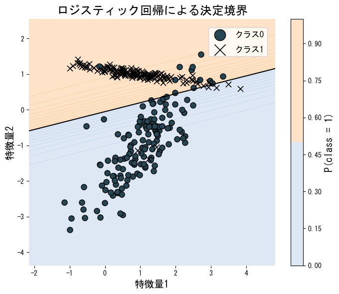
ロジスティック回帰は決定境界が線形であるため、非線形な分布のデータにはそのまま適用できません。多項式特徴量やカーネル近似を組み合わせるか、SVMやニューラルネットワークなどの非線形モデルを検討してください。
係数の絶対値が大きい特徴量ほど予測への影響が大きいですが、スケールが揃っていないと比較できません。StandardScalerで標準化したうえで係数を比較してください。多クラス分類ではソフトマックス回帰に拡張できます。
罰則 C と決定境界 #
罰則係数 C を変えるとロジスティック回帰の決定境界がどう変化するか確認できます。
まとめ #
- ロジスティック回帰はシグモイド関数を用いて、入力に対するクラス1の確率を直接推定します。
- 出力が確率として解釈できるため、しきい値を調整してPrecision/Recallのトレードオフを制御できます。
- L1/L2正則化を組み合わせることで、過学習の抑制と不要な特徴量の除去が可能です。
- 決定境界が線形であるため、解釈性が高い反面、非線形な分布には対応できない点に注意が必要です。
参考文献 #
- Agresti, A. (2015). Foundations of Linear and Generalized Linear Models. Wiley.
- Hastie, T., Tibshirani, R., & Friedman, J. (2009). The Elements of Statistical Learning. Springer.