パーセプトロン | 最もシンプルな線形分類器

まとめ

パーセプトロンは線形に分離可能なデータで有限回の更新で収束する、古典的なオンライン学習アルゴリズムです。
重み付き和 $\mathbf{w}^\top \mathbf{x} + b$ の符号だけで予測でき、誤分類したサンプルでのみ重みを更新します。
更新則が単純なため勾配法の直感をつかみやすく、学習率を調整しながら決定境界を少しずつ動かします。
非線形データにはそのままでは対応できないため、特徴量拡張やカーネルトリックと組み合わせます。

直感 #

パーセプトロンは「誤分類したら境界をサンプルのある側へ少し動かす」という素朴な考え方で学習します。重みベクトル $\mathbf{w}$ は決定境界の法線方向を表し、バイアス $b$ がオフセットを表します。学習率 $\eta$ を調整しながら境界を動かすと、誤りが減る方向へ徐々に収束します。

数式で見る #

予測は

$$ \hat{y} = \operatorname{sign}(\mathbf{w}^\top \mathbf{x} + b) $$

で行います。サンプル $(\mathbf{x}_i, y_i)$ を誤分類した場合、以下のように更新します。

$$ \mathbf{w} \leftarrow \mathbf{w} + \eta, y_i, \mathbf{x}_i,\qquad b \leftarrow b + \eta, y_i $$

データが線形に分離可能であれば、この更新を繰り返すだけで有限回で収束することが知られています。

Pythonによる実験 #

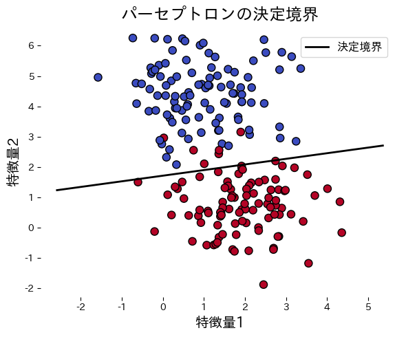
次のコードは人工データにパーセプトロンを適用し、学習の進み具合と決定境界を可視化する例です。誤分類が 0 になった時点で更新を打ち切ります。

from __future__ import annotations

import japanize_matplotlib
import matplotlib.pyplot as plt
import numpy as np
from sklearn.datasets import make_blobs
from sklearn.metrics import accuracy_score


def run_perceptron_demo(
    n_samples: int = 200,
    lr: float = 0.1,
    n_epochs: int = 20,
    random_state: int = 0,
    title: str = "パーセプトロンの決定境界",
    xlabel: str = "特徴量1",
    ylabel: str = "特徴量2",
    label_boundary: str = "決定境界",
) -> dict[str, object]:
    """Train a perceptron on synthetic blobs and plot the decision boundary."""
    japanize_matplotlib.japanize()
    X, y = make_blobs(
        n_samples=n_samples,
        centers=2,
        cluster_std=1.0,
        random_state=random_state,
    )
    y_signed = np.where(y == 0, -1, 1)

    w = np.zeros(X.shape[1])
    b = 0.0
    history: list[int] = []

    for _ in range(n_epochs):
        errors = 0
        for xi, target in zip(X, y_signed):
            update = lr * target if target * (np.dot(w, xi) + b) <= 0 else 0.0
            if update != 0.0:
                w += update * xi
                b += update
                errors += 1
        history.append(int(errors))
        if errors == 0:
            break

    preds = np.where(np.dot(X, w) + b >= 0, 1, -1)
    accuracy = float(accuracy_score(y_signed, preds))

    xx = np.linspace(X[:, 0].min() - 1, X[:, 0].max() + 1, 200)
    yy = -(w[0] * xx + b) / w[1]

    fig, ax = plt.subplots(figsize=(6, 5))
    ax.scatter(X[:, 0], X[:, 1], c=y, cmap="coolwarm", edgecolor="k")
    ax.plot(xx, yy, color="black", linewidth=2, label=label_boundary)
    ax.set_xlabel(xlabel)
    ax.set_ylabel(ylabel)
    ax.set_title(title)
    ax.legend(loc="best")
    fig.tight_layout()
    plt.show()

    return {"weights": w, "bias": b, "errors": history, "accuracy": accuracy}


metrics = run_perceptron_demo(
    title="パーセプトロンの決定境界",
    xlabel="特徴量1",
    ylabel="特徴量2",
    label_boundary="決定境界",
)
print(f"訓練精度: {metrics['accuracy']:.3f}")
print("重み:", metrics['weights'])
print(f"バイアス: {metrics['bias']:.3f}")
print("各エポックの誤り数:", metrics['errors'])

誤分類が 0 になった時点で更新を打ち切りますの図

参考文献 #

Rosenblatt, F. (1958). The Perceptron: A Probabilistic Model for Information Storage and Organization in the Brain. Psychological Review, 65(6), 386 E08.
Goodfellow, I., Bengio, Y., & Courville, A. (2016). Deep Learning. MIT Press.