2.2.2
ソフトマックス回帰
まとめ
- ソフトマックス回帰はロジスティック回帰を多クラスへ拡張し、すべてのクラスの出現確率を同時に推定します。
- 出力は 0 以上 1 以下で総和が 1 になるため、しきい値設定やコスト計算にそのまま利用できます。
- 学習はクロスエントロピー損失を最小化することで行い、予測確率と真の分布のずれを直接補正します。
- scikit-learn では
LogisticRegression(multi_class="multinomial")がソフトマックス回帰を実装し、L1/L2 正則化にも対応しています。
- ロジスティック回帰 の概念を先に学ぶと理解がスムーズです
直感 #
二値分類ではシグモイド関数がクラス1の確率を返しますが、多クラス問題では「すべてのクラスの確率を同時に知りたい」ときが多くあります。ソフトマックス回帰はクラスごとの線形スコアを指数関数で変換し、それらを正規化して確率分布にします。スコアの高いクラスが強調され、低いクラスは抑えられます。
flowchart LR
A["入力x"] --> B["クラスごとの\n線形スコア"]
B --> C["exp変換"]
C --> D["正規化\n(総和=1)"]
D --> E["確率分布\nP(y=k|x)"]
E --> F["argmax\n→予測クラス"]
style A fill:#2563eb,color:#fff
style D fill:#1e40af,color:#fff
style F fill:#10b981,color:#fff
数式で見る #
クラス数を \(K\)、クラス \(k\) の重みベクトルとバイアスをそれぞれ \(\mathbf{w}_k\)、\(b_k\) とすると
$$ P(y = k \mid \mathbf{x}) = \frac{\exp\left(\mathbf{w}_k^\top \mathbf{x} + b_k\right)} {\sum_{j=1}^{K} \exp\left(\mathbf{w}_j^\top \mathbf{x} + b_j\right)} $$で確率が得られます。目的関数はクロスエントロピー損失
$$ L = - \sum_{i=1}^{n} \sum_{k=1}^{K} \mathbb{1}(y_i = k) \log P(y = k \mid \mathbf{x}_i) $$です。重みに正則化項を加えると過学習を抑えられます。
Pythonによる実験 #
下記は3クラスの人工データにソフトマックス回帰を適用し、決定領域を描画した例です。multi_class="multinomial" を指定するとソフトマックス学習が有効になります。
| |
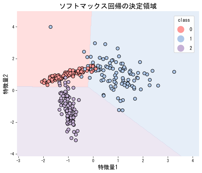
ソフトマックス回帰の決定境界は線形です。クラス間の境界が非線形な場合は、多項式特徴量を追加するか、SVMやニューラルネットワークなどの非線形モデルを検討してください。
scikit-learnのLogisticRegressionはデフォルトでsolver="lbfgs"を使い安定して収束します。特徴量が非常に多い場合はsolver="saga"とL1正則化(penalty="l1")を組み合わせると、不要な特徴量の重みを0にして解釈性を高められます。
温度と決定境界 #
温度パラメータを変えるとソフトマックスの決定境界の鋭さがどう変化するか確認できます。
まとめ #
- ソフトマックス回帰はロジスティック回帰を多クラスへ拡張し、各クラスの出現確率を同時に推定します。
- 出力は0以上1以下で総和が1になるため、確率として直接利用できます。
- クロスエントロピー損失を最小化して学習し、L1/L2正則化で過学習を抑制できます。
- 決定境界が線形であるため解釈性は高いですが、非線形な分布には対応できない点に注意が必要です。
参考文献 #
- Bishop, C. M. (2006). Pattern Recognition and Machine Learning. Springer.
- Murphy, K. P. (2012). Machine Learning: A Probabilistic Perspective. MIT Press.