DBSCAN | 密度の違いからクラスタを抽出する

まとめ

DBSCAN（Density-Based Spatial Clustering of Applications with Noise）は、密度が高い領域をクラスタ、疎な領域をノイズとして扱うアルゴリズムです。
距離の半径 eps と近傍に必要な点数 min_samples を指定し、点をコア・境界・ノイズの 3 種類に分類します。
クラスタ数を事前に決める必要がなく、非凸な形のクラスタやノイズを含むデータに強いのが特徴です。
min_samples-距離プロットを手掛かりに eps を調整し、距離のスケールを揃えるために標準化しておくと安定します。

直感 #

DBSCAN は「点の周囲に十分な仲間がいるかどうか」を基準にクラスタを構成します。

コアポイント: 半径 eps の円内に min_samples 個以上の点がある点。
境界ポイント: コアポイントの近傍に存在するが、自分自身は条件を満たさない点。
ノイズ: コアにも境界にも分類されない孤立した点。

コアポイント同士が鎖のようにつながると同じ密度領域として扱われ、その領域が 1 つのクラスタになります。クラスタの形が不規則でも対応できますが、密度差が大きいデータではパラメータ調整が重要です。

数式で見る #

データ集合 $\mathcal{X}$ の点 $x_i$ に対し、eps で定義される $\varepsilon$-近傍は

$$ \mathcal{N}_\varepsilon(x_i) = {, x_j \in \mathcal{X} \mid \lVert x_i - x_j \rVert \le \varepsilon ,} $$

です。近傍に十分な点が存在すればコアポイントになります。

$$ |\mathcal{N}_\varepsilon(x_i)| \ge \texttt{min_samples} $$

コアポイント同士が密度連結であれば同じクラスタに属し、境界ポイントはクラスタにぶら下がる形で所属します。ノイズはどのクラスタにも属さない点です。

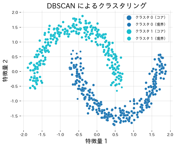
Pythonで確かめる #

標準化した月型データに DBSCAN を適用し、クラスタ数とノイズ点の数を確認します。

from __future__ import annotations

import japanize_matplotlib
import matplotlib.pyplot as plt
import numpy as np
from numpy.typing import NDArray
from sklearn.cluster import DBSCAN
from sklearn.datasets import make_moons
from sklearn.preprocessing import StandardScaler


def run_dbscan_demo(
    n_samples: int = 600,
    noise: float = 0.08,
    eps: float = 0.3,
    min_samples: int = 10,
    random_state: int = 0,
) -> dict[str, int]:
    """DBSCAN で月型データをクラスタリングし、クラスタ数とノイズ点を調べる。"""
    japanize_matplotlib.japanize()
    features, _ = make_moons(
        n_samples=n_samples,
        noise=noise,
        random_state=random_state,
    )
    features = StandardScaler().fit_transform(features)

    model = DBSCAN(eps=eps, min_samples=min_samples)
    labels = model.fit_predict(features)

    unique_labels = sorted(np.unique(labels))
    cluster_ids = [label for label in unique_labels if label != -1]
    noise_count = int(np.sum(labels == -1))

    core_mask = np.zeros(labels.shape[0], dtype=bool)
    if hasattr(model, "core_sample_indices_"):
        core_mask[model.core_sample_indices_] = True

    fig, ax = plt.subplots(figsize=(6.2, 5.2))
    palette = plt.cm.get_cmap("tab10", max(len(cluster_ids), 1))

    for order, cluster_id in enumerate(cluster_ids):
        mask = labels == cluster_id
        color = palette(order)
        ax.scatter(
            features[mask & core_mask, 0],
            features[mask & core_mask, 1],
            c=[color],
            s=36,
            edgecolor="white",
            linewidth=0.2,
            label=f"クラスタ {cluster_id}（コア）",
        )
        ax.scatter(
            features[mask & ~core_mask, 0],
            features[mask & ~core_mask, 1],
            c=[color],
            s=24,
            edgecolor="white",
            linewidth=0.2,
            marker="o",
            label=f"クラスタ {cluster_id}（境界）",
        )

    if noise_count:
        noise_mask = labels == -1
        ax.scatter(
            features[noise_mask, 0],
            features[noise_mask, 1],
            c="#9ca3af",
            marker="x",
            s=28,
            linewidth=0.8,
            label="ノイズ",
        )

    ax.set_title("DBSCAN によるクラスタリング")
    ax.set_xlabel("特徴量 1")
    ax.set_ylabel("特徴量 2")
    ax.grid(alpha=0.2)
    ax.legend(loc="upper right", fontsize=9)
    fig.tight_layout()
    plt.show()

    return {"n_clusters": len(cluster_ids), "n_noise": noise_count}


result = run_dbscan_demo()
print(f"検出されたクラスタ数: {result['n_clusters']}")
print(f"ノイズ点の数: {result['n_noise']}")

標準化した月型データに DBSCAN を適用し、クラスタ数とノイズ点の数を確認しますの図

参考文献 #

Ester, M., Kriegel, H.-P., Sander, J., & Xu, X. (1996). A Density-Based Algorithm for Discovering Clusters in Large Spatial Databases with Noise. KDD.
Schubert, E., Sander, J., Ester, M., Kriegel, H.-P., & Xu, X. (2017). DBSCAN Revisited, Revisited. ACM Transactions on Database Systems.
scikit-learn developers. (2024). Clustering. https://scikit-learn.org/stable/modules/clustering.html