ガウス混合モデル (GMM) | 確率クラスタリングとソフト割り当て

まとめ

ガウス混合モデルは複数の多変量正規分布を重ね合わせ、データ全体の確率分布を表す生成モデルです。
各サンプルに対してクラスタ所属確率（責務）が推定でき、ハードな割り当てでは見えない曖昧さを表現できます。
パラメータは EM アルゴリズムで推定し、分散共分散行列の形を full, tied, diag, spherical から選択できます。
BIC や AIC を使ったモデル選択、複数回の初期化による安定化が実務では不可欠です。

直感 #

「データは複数のガウス分布が混ざったもの」と仮定すると、各クラスタは平均ベクトルと共分散行列を持つ楕円体として表現できます。k-means が最も近いクラスタを 1 つだけ返すのに対し、GMM は「クラスタ $k$ がサンプル $x_i$ を生み出した確率 $\gamma_{ik}$」を返すソフトクラスタリングを行います。

数式 #

入力ベクトル $\mathbf{x}$ の確率密度は

$$ p(\mathbf{x}) = \sum_{k=1}^{K} \pi_k , \mathcal{N}(\mathbf{x} \mid \boldsymbol{\mu}_k, \boldsymbol{\Sigma}_k), $$

で表されます。$\pi_k$ は混合係数（非負で総和が 1）、$\boldsymbol{\mu}_k$ は平均、$\boldsymbol{\Sigma}_k$ は共分散行列です。EM アルゴリズムでは以下を収束まで繰り返します。

E-step: 責務 $\gamma_{ik}$ を求める。 $$ \gamma_{ik} = \frac{\pi_k , \mathcal{N}(\mathbf{x}_i \mid \boldsymbol{\mu}_k, \boldsymbol{\Sigma}k)} {\sum{j=1}^K \pi_j , \mathcal{N}(\mathbf{x}_i \mid \boldsymbol{\mu}_j, \boldsymbol{\Sigma}_j)}. $$
M-step: 責務を重みとして $\pi_k, \boldsymbol{\mu}_k, \boldsymbol{\Sigma}_k$ を更新。

対数尤度は単調に増加し、局所最大に収束します。

Pythonで確かめる #

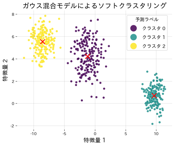
合成データに GMM を適用し、クラスタ中心と責務を可視化します。

from __future__ import annotations

import japanize_matplotlib
import matplotlib.pyplot as plt
import numpy as np
from numpy.typing import NDArray
from sklearn.datasets import make_blobs
from sklearn.mixture import GaussianMixture


def run_gmm_demo(
    n_samples: int = 600,
    n_components: int = 3,
    cluster_std: list[float] | tuple[float, ...] = (1.0, 1.4, 0.8),
    covariance_type: str = "full",
    random_state: int = 7,
    n_init: int = 8,
) -> dict[str, object]:
    """ガウス混合モデルを学習し、責務とクラスタ中心を可視化する。"""
    japanize_matplotlib.japanize()
    features, labels_true = make_blobs(
        n_samples=n_samples,
        centers=n_components,
        cluster_std=cluster_std,
        random_state=random_state,
    )

    gmm = GaussianMixture(
        n_components=n_components,
        covariance_type=covariance_type,
        random_state=random_state,
        n_init=n_init,
    )
    gmm.fit(features)

    hard_labels = gmm.predict(features)
    responsibilities = gmm.predict_proba(features)
    log_likelihood = float(gmm.score(features))
    weights = gmm.weights_

    fig, ax = plt.subplots(figsize=(6.2, 5.2))
    scatter = ax.scatter(
        features[:, 0],
        features[:, 1],
        c=hard_labels,
        cmap="viridis",
        s=30,
        edgecolor="white",
        linewidth=0.2,
        alpha=0.85,
    )
    ax.scatter(
        gmm.means_[:, 0],
        gmm.means_[:, 1],
        marker="x",
        c="red",
        s=140,
        linewidth=2.0,
        label="クラスタ中心",
    )
    ax.set_title("ガウス混合モデルによるソフトクラスタリング")
    ax.set_xlabel("特徴量 1")
    ax.set_ylabel("特徴量 2")
    ax.grid(alpha=0.2)
    handles, _ = scatter.legend_elements()
    labels = [f"クラスタ {idx}" for idx in range(n_components)]
    ax.legend(handles, labels, title="予測ラベル", loc="upper right")
    fig.tight_layout()
    plt.show()

    return {
        "log_likelihood": log_likelihood,
        "weights": weights.tolist(),
        "responsibilities_shape": responsibilities.shape,
    }


metrics = run_gmm_demo()
print(f"対数尤度: {metrics['log_likelihood']:.3f}")
print("混合係数:", metrics["weights"])
print("責務行列の形状:", metrics["responsibilities_shape"])

合成データに GMM を適用し、クラスタ中心と責務を可視化しますの図

参考文献 #

Bishop, C. M. (2006). Pattern Recognition and Machine Learning. Springer.
Dempster, A. P., Laird, N. M., & Rubin, D. B. (1977). Maximum Likelihood from Incomplete Data via the EM Algorithm. Journal of the Royal Statistical Society, Series B.
scikit-learn developers. (2024). Gaussian Mixture Models. https://scikit-learn.org/stable/modules/mixture.html