k-means

入門

2.5.1

k-means

最終更新 2020-01-29 読了時間 3 分

まとめ

k-meansは「距離が近い点同士をまとめる」という直感をもとに、セントロイド（重心）を反復更新してデータを $k$ 個に分割する。
目的関数は各サンプルと所属クラスターのセントロイドとの距離二乗和（WCSS）で、これを最小にする配置を探す。
クラスター数 $k$ の選択にはエルボー法やシルエット係数を使い、データ構造とビジネス要件を踏まえて判断する。

直感 #

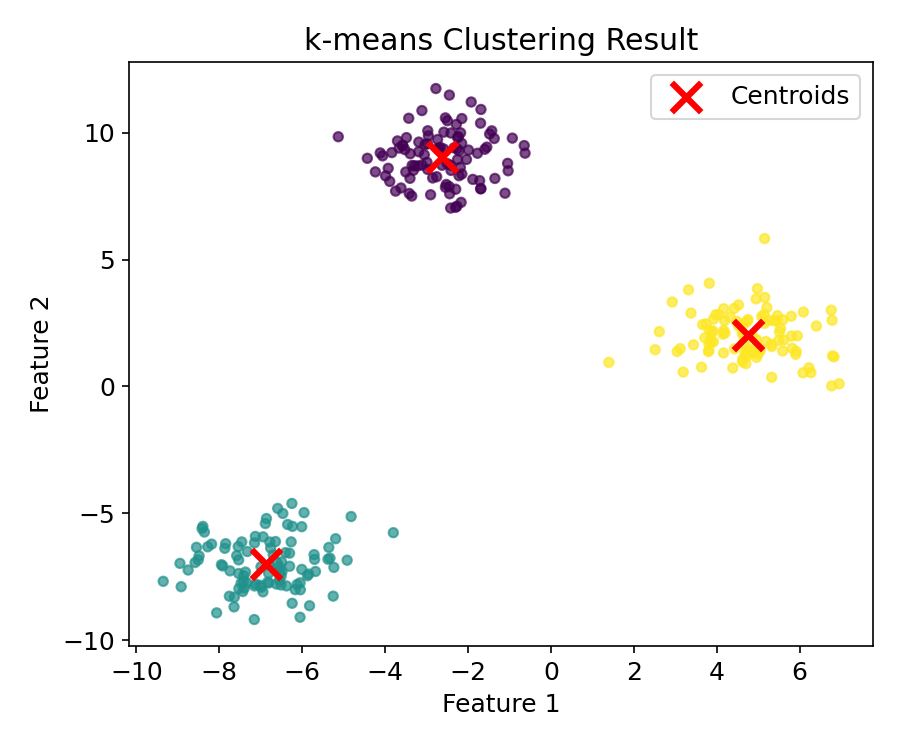
k-meansは教師なし学習のもっとも基本的なクラスターリング手法です。$k$ 個のセントロイドをランダムに配置し、「各点をもっとも近いセントロイドに割り当てる」→「セントロイドをクラスターの平均に移動する」を収束するまで繰り返す。アルゴリズムは単純だが、初期値や $k$ の選び方で結果が変わるため、適切な評価指標と組み合わせて使う必要がある。

flowchart LR A["データX"] --> B["k個の\nセントロイド初期化"] B --> C["各点を最近の\nセントロイドに割当"] C --> D["セントロイドを\nクラスター平均に更新"] D --> E{"収束？"} E -->|No| C E -->|Yes| F["最終クラスター"] style A fill:#2563eb,color:#fff style D fill:#1e40af,color:#fff style F fill:#10b981,color:#fff

アルゴリズムの詳細 #

目的関数 #

k-meansはWCSS（Within-Cluster Sum of Squares）、すなわち各サンプルと所属クラスターのセントロイドとの距離二乗和を最小化します。

$$ J = \sum_{k=1}^{K} \sum_{\mathbf{x}_i \in C_k} \lVert \mathbf{x}_i - \boldsymbol{\mu}_k \rVert^2 $$

ここで$C_k$はクラスター$k$に属するサンプルの集合、$\boldsymbol{\mu}_k$はクラスター$k$のセントロイドです。この目的関数はNP困難ですが、以下の2ステップを交互に繰り返すことで局所最適解に収束します。

Lloyd のアルゴリズム #

割り当てステップ: 各サンプル$\mathbf{x}_i$をもっとも近いセントロイドのクラスターに割り当てます。
$$ c_i = \arg\min_{k} \lVert \mathbf{x}_i - \boldsymbol{\mu}_k \rVert^2 $$
更新ステップ: 各クラスターのセントロイドを、そのクラスターに属するサンプルの平均に更新します。
$$ \boldsymbol{\mu}_k = \frac{1}{|C_k|} \sum_{\mathbf{x}_i \in C_k} \mathbf{x}_i $$
割り当てが変化しなくなるまで1–2を繰り返します。

収束の保証 #

各ステップで目的関数$J$は単調に減少します。

割り当てステップでは、各サンプルをもっとも近いセントロイドに再割り当てするため、$J$は減少または不変です
更新ステップでは、クラスター内の平均がユークリッド距離の二乗和を最小にする点であるため、$J$は減少または不変です

$J$は下に有界（$J \ge 0$）かつ単調非増加であるため、有限回のステップで収束が保証されます。ただし、収束先は大域的最適解とは限りません。

k-means++ 初期化 #

ランダム初期化では悪い局所解に陥りやすいため、k-means++では初期セントロイドを以下の手順で選びます。

最初のセントロイド$\boldsymbol{\mu}_1$をデータからランダムに選びます
各サンプル$\mathbf{x}_i$について、もっとも近い既存セントロイドとの距離$D(\mathbf{x}_i)$を計算します
$D(\mathbf{x}_i)^2$に比例する確率で次のセントロイドを選びます
$K$個のセントロイドが選ばれるまで2–3を繰り返します

この初期化により、期待値で$O(\log K)$倍以内の近似が保証されます。

$$ \mathbb{E}[J_{\text{k-means++}}] \le 8(\ln K + 2) \cdot J_{\text{opt}} $$

flowchart TD A["k-means++ で\nセントロイド初期化"] --> B["割り当てステップ\nc_i = argmin ||x_i − μ_k||²"] B --> C["更新ステップ\nμ_k = mean(C_k)"] C --> D{"割り当て\n変化あり？"} D -->|Yes| B D -->|No| E["収束: 局所最適解"] E --> F["n_init 回繰り返し\n最小 J を採用"] style A fill:#2563eb,color:#fff style B fill:#1e40af,color:#fff style F fill:#10b981,color:#fff

参考リンク

Lloyd, S. (1982). Least squares quantization in PCM. IEEE Transactions on Information Theory, 28(2), 129–137.

Arthur, D., & Vassilvitskii, S. (2007). k-means++: The Advantages of Careful Seeding. Proceedings of the 18th Annual ACM-SIAM Symposium on Discrete Algorithms (SODA), 1027–1035.

詳細な解説 #

ライブラリと実験データ #

1
2
3
4
5
import numpy as np
import matplotlib.pyplot as plt
from sklearn.datasets import make_blobs
from sklearn.cluster import KMeans
from sklearn.metrics import silhouette_score

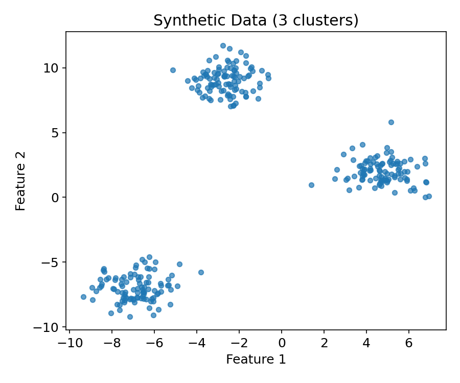
3つの塊を持つ合成データを生成します。

1
2
3
4
5
6
7
8
9
X, y_true = make_blobs(
    n_samples=300, centers=3,
    cluster_std=1.0, random_state=42
)

plt.figure(figsize=(6, 5))
plt.scatter(X[:, 0], X[:, 1], s=20, alpha=0.7)
plt.title("合成データ（3クラスター）")
plt.show()

合成データの散布図

基本的な学習 #

 1
 2
 3
 4
 5
 6
 7
 8
 9
10
11
12
13
kmeans = KMeans(n_clusters=3, random_state=42, n_init=10)
labels = kmeans.fit_predict(X)

plt.figure(figsize=(6, 5))
plt.scatter(X[:, 0], X[:, 1], c=labels, cmap="viridis", s=20, alpha=0.7)
plt.scatter(
    kmeans.cluster_centers_[:, 0],
    kmeans.cluster_centers_[:, 1],
    c="red", marker="x", s=200, linewidths=3, label="セントロイド",
)
plt.legend()
plt.title("k-means クラスターリング結果")
plt.show()

k-meansクラスターリング結果

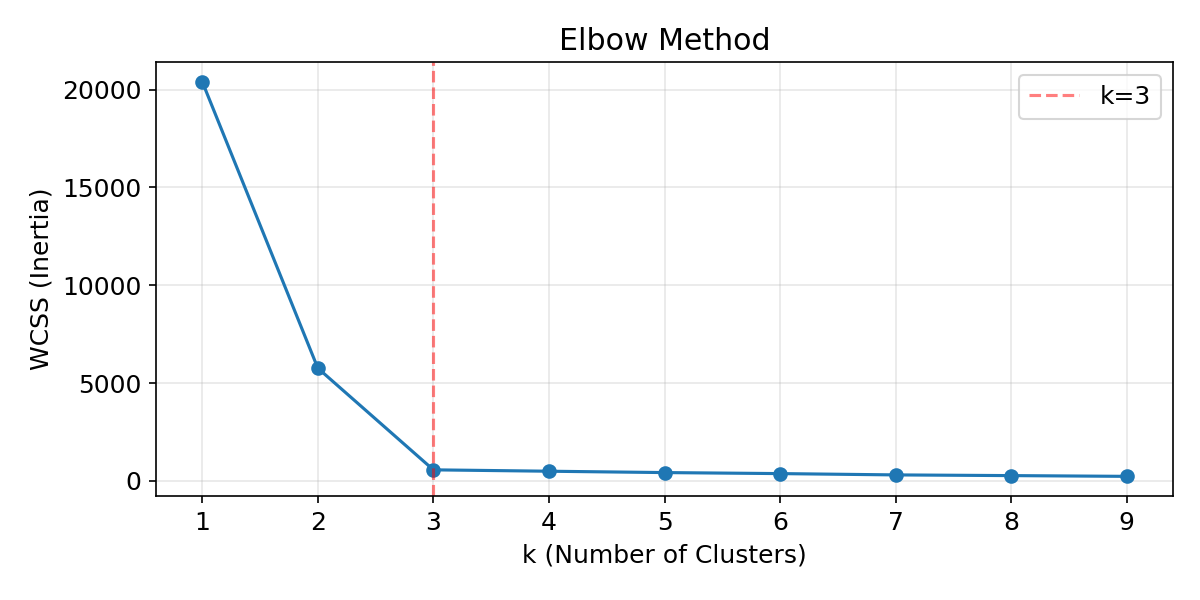
エルボー法でクラスター数を選ぶ #

WCSS（Within-Cluster Sum of Squares）を $k$ ごとに計算し、減少が鈍化する「肘」の位置を $k$ の候補とします。

 1
 2
 3
 4
 5
 6
 7
 8
 9
10
11
12
13
14
inertias = []
K_range = range(1, 10)
for k in K_range:
    km = KMeans(n_clusters=k, random_state=42, n_init=10)
    km.fit(X)
    inertias.append(km.inertia_)

plt.figure(figsize=(8, 4))
plt.plot(K_range, inertias, "o-")
plt.xlabel("k（クラスター数）")
plt.ylabel("WCSS（慣性）")
plt.title("エルボー法")
plt.grid(True)
plt.show()

エルボー法によるk選択

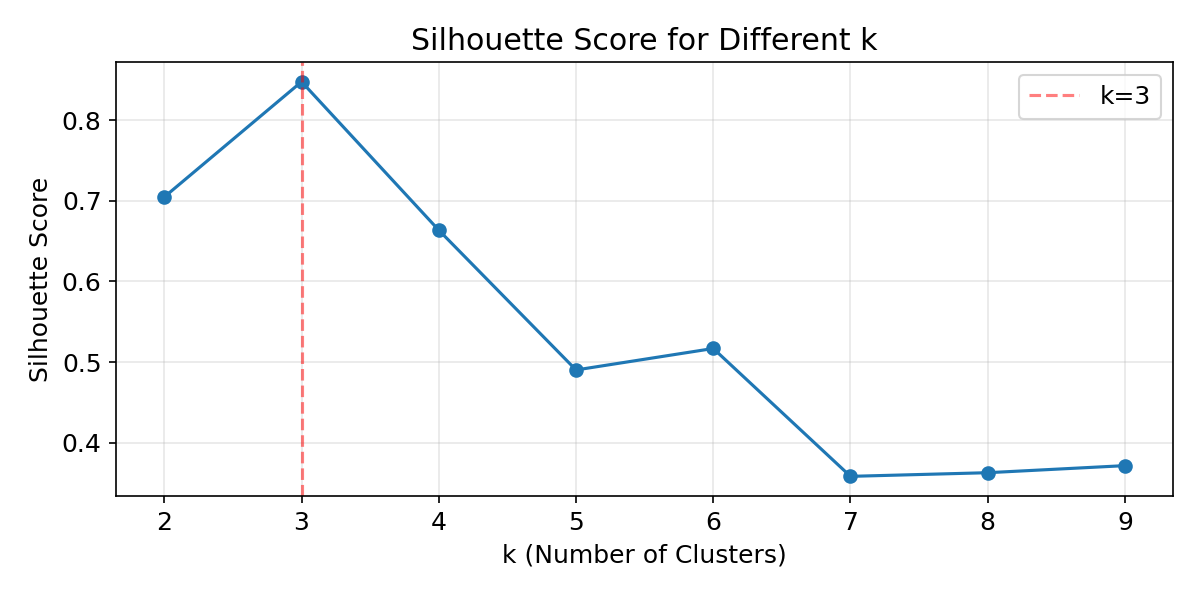
シルエット係数でクラスター数を評価 #

シルエット係数はクラスターの凝集度と分離度のバランスを測ります。1に近いほどクラスターが明確に分かれていることを示します。

 1
 2
 3
 4
 5
 6
 7
 8
 9
10
11
12
13
14
sil_scores = []
K_range2 = range(2, 10)
for k in K_range2:
    km = KMeans(n_clusters=k, random_state=42, n_init=10)
    labels_k = km.fit_predict(X)
    sil_scores.append(silhouette_score(X, labels_k))

plt.figure(figsize=(8, 4))
plt.plot(K_range2, sil_scores, "o-")
plt.xlabel("k（クラスター数）")
plt.ylabel("シルエット係数")
plt.title("シルエット係数によるk選択")
plt.grid(True)
plt.show()

シルエット係数によるk選択

n_initの役割 #

k-meansはランダムな初期値に依存するため、n_init回の試行から最良の結果を採用します。

1
2
3
4
5
6
results = []
for n in [1, 3, 10, 30]:
    km = KMeans(n_clusters=3, random_state=42, n_init=n)
    km.fit(X)
    results.append((n, km.inertia_))
    print(f"n_init={n:2d}  WCSS={km.inertia_:.2f}")

k-meansはクラスターが球状で等分散であることを仮定しています。三日月型や密度が大きく異なるクラスターには適用できません。また、特徴量のスケールが異なる場合はStandardScalerで標準化してから適用してください。

エルボー法だけでは「肘」の位置が曖昧なことがあります。シルエット係数と併用し、複数の指標で $k$ を判断するのが実務的です。n_init=10以上に設定して初期値依存を減らすことも忘れずに行ってください。

まとめ #

k-meansはセントロイドの割り当てと更新を繰り返すことで、データを $k$ 個のクラスターに分割します。
エルボー法やシルエット係数を使って、適切なクラスター数 $k$ を定量的に選択できます。
初期値に依存するため、n_initパラメーターで複数回の試行から最良の結果を採用します。
球状クラスターを仮定するため、非凸な形状のクラスターにはDBSCANなど密度ベースの手法が適しています。

k-means++ — 初期セントロイドを賢く選ぶ改良版
X-means — クラスター数を自動で推定する発展手法
DBSCAN — 密度ベースのクラスターリング