まとめ AdaBoost分類は誤分類されたサンプルに重みを寄せながら弱学習器を逐次学習し、最終的に重み付き多数決で分類する。 learning_rate と n_estimators の組み合わせで、過学習と未学習のバランスを調整できる。弱学習器に浅い決定木を使うことで、境界が複雑なデータでも段階的に性能を引き上げられる。 決定木分類器 — AdaBoost は決定木を弱学習器として使います
直感
# AdaBoost分類の本質は『前段で間違えた点を次段で重点的に学ぶ』ことです。1本ずつは弱い分類器でも、誤りに応じて重み付けして合成すると、難しい境界を徐々に補正できる強い分類器になります。
数学的定式化
# アルゴリズムの流れ
# 2 クラス分類を例に説明します。ラベルを $y_i \in {-1, +1}$ とし、$N$ 個の訓練データに対して初期重みを均等に設定します。
$$w_i^{(1)} = \frac{1}{N}, \quad i = 1, \dots, N$$各ラウンド $t = 1, \dots, T$ で以下を繰り返します。
Step 1. 弱学習器の学習 — 重み $w^{(t)}$ のもとで弱分類器 $h_t(x)$ を学習する。
Step 2. 加重誤差率の計算
$$\epsilon_t = \sum_{i=1}^{N} w_i^{(t)} \cdot \mathbb{1}[h_t(x_i) \neq y_i]$$$\epsilon_t$ は重み付き誤分類率です。$\epsilon_t < 0.5$(ランダムより良い)であれば、この弱学習器は価値があります。
Step 3. 分類器重みの計算
$$\alpha_t = \frac{1}{2} \ln \frac{1 - \epsilon_t}{\epsilon_t}$$$\epsilon_t$ が小さいほど $\alpha_t$ は大きくなり、その弱学習器の発言力が強まります。
Step 4. サンプル重みの更新
$$w_i^{(t+1)} = \frac{w_i^{(t)} \cdot \exp(-\alpha_t \, y_i \, h_t(x_i))}{Z_t}$$ここで $Z_t$ は正規化定数(重みの総和を 1 にする)です。
正解した点: $y_i h_t(x_i) = +1$ → 重みが小さく なる 誤分類した点: $y_i h_t(x_i) = -1$ → 重みが大きく なる 最終決定関数
# $T$ ラウンド後の最終予測は、全弱学習器の重み付き多数決です。
$$H(x) = \text{sign}\!\left(\sum_{t=1}^{T} \alpha_t \, h_t(x)\right)$$指数損失との関係
# AdaBoost は指数損失 を暗黙的に最小化していることが知られています。
$$L_{\exp} = \sum_{i=1}^{N} \exp\!\left(-y_i \sum_{t=1}^{T} \alpha_t h_t(x_i)\right)$$$F(x) = \sum_t \alpha_t h_t(x)$ に対して関数空間上での勾配降下法を行うと、AdaBoost の更新則と一致します。この解釈から、AdaBoost はブースティング=加法モデルの逐次最適化 という統一的な枠組みに位置付けられます。
flowchart LR
A["初期重み\nw = 1/N"] --> B["弱学習器を学習\nh_t(x)"]
B --> C["加重誤差率\nε_t を計算"]
C --> D["分類器重み\nα_t を計算"]
D --> E["サンプル重み\n更新"]
E -->|"t < T"| B
E -->|"t = T"| F["重み付き多数決\nH(x) = sign(Σα_t h_t)"]
style A fill:#2563eb,color:#fff
style F fill:#10b981,color:#fff
詳細な解説
# 1
2
3
4
5
6
7
8
import matplotlib.pyplot as plt
import numpy as np
from sklearn.datasets import make_classification
from sklearn.model_selection import train_test_split
from sklearn.metrics import roc_auc_score
from sklearn.tree import DecisionTreeClassifier
from sklearn.ensemble import AdaBoostClassifier
実験用のデータを作成
# 1
2
3
4
5
6
7
8
9
10
11
12
13
# 特徴が20あるデータを作成
n_features = 20
X , y = make_classification (
n_samples = 2500 ,
n_features = n_features ,
n_informative = 10 ,
n_classes = 2 ,
n_redundant = 4 ,
n_clusters_per_class = 5 ,
)
X_train , X_test , y_train , y_test = train_test_split (
X , y , test_size = 0.33 , random_state = 42
)
Adaboostモデルを訓練
# 1
2
3
4
5
6
7
8
9
10
11
12
ab_clf = AdaBoostClassifier (
n_estimators = 10 ,
learning_rate = 1.0 ,
random_state = 117117 ,
base_estimator = DecisionTreeClassifier ( max_depth = 2 ),
)
ab_clf . fit ( X_train , y_train )
y_pred = ab_clf . predict ( X_test )
ab_clf_score = roc_auc_score ( y_test , y_pred )
ab_clf_score
0.7546477034876885
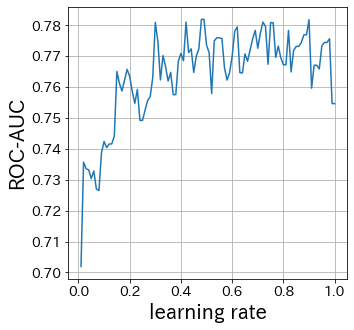
learning-rateの影響
# learning-rateが小さければ小さいほど重みの更新幅は小さくなります。逆に大きすぎると、収束しない場合があります。
1
2
3
4
5
6
7
8
9
10
11
12
13
scores = []
learning_rate_list = np . linspace ( 0.01 , 1 , 100 )
for lr in learning_rate_list :
ab_clf_i = AdaBoostClassifier (
n_estimators = 10 ,
learning_rate = lr ,
random_state = 117117 ,
base_estimator = DecisionTreeClassifier ( max_depth = 2 ),
)
ab_clf_i . fit ( X_train , y_train )
y_pred = ab_clf_i . predict ( X_test )
scores . append ( roc_auc_score ( y_test , y_pred ))
1
2
3
4
5
6
plt . figure ( figsize = ( 5 , 5 ))
plt . plot ( learning_rate_list , scores )
plt . xlabel ( "learning rate" )
plt . ylabel ( "ROC-AUC" )
plt . grid ()
plt . show ()
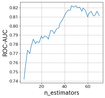
n_estimatorsの影響
# n_estimatorsは弱学習器の数を指定しています。
通常は、このパラメタを大きくしたり小さくしたりする必要はないです。
ある程度大きな数でn_estimatorsを固定して、そのあとで他のパラメタを調整します。
 1
 2
 3
 4
 5
 6
 7
 8
 9
10
11
12
13
scores = []
n_estimators_list = [ int ( ne ) for ne in np . linspace ( 5 , 70 , 40 )]
for n_estimators in n_estimators_list :
ab_clf_i = AdaBoostClassifier (
n_estimators = int ( n_estimators ),
learning_rate = 0.6 ,
random_state = 117117 ,
base_estimator = DecisionTreeClassifier ( max_depth = 2 ),
)
ab_clf_i . fit ( X_train , y_train )
y_pred = ab_clf_i . predict ( X_test )
scores . append ( roc_auc_score ( y_test , y_pred ))
1
2
3
4
5
6
plt . figure ( figsize = ( 5 , 5 ))
plt . plot ( n_estimators_list , scores )
plt . xlabel ( "n_estimators" )
plt . ylabel ( "ROC-AUC" )
plt . grid ()
plt . show ()
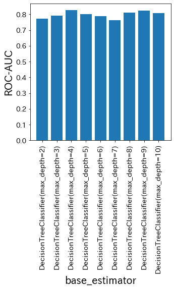
base-estimatorの影響
# base-estimatorは弱学習器として何を使用するか指定します。つまり、Adaboostで最も重要なパラメタの一つです。
 1
 2
 3
 4
 5
 6
 7
 8
 9
10
11
12
13
14
15
scores = []
base_estimator_list = [
DecisionTreeClassifier ( max_depth = md ) for md in [ 2 , 3 , 4 , 5 , 6 , 7 , 8 , 9 , 10 ]
]
for base_estimator in base_estimator_list :
ab_clf_i = AdaBoostClassifier (
n_estimators = 10 ,
learning_rate = 0.5 ,
random_state = 117117 ,
base_estimator = base_estimator ,
)
ab_clf_i . fit ( X_train , y_train )
y_pred = ab_clf_i . predict ( X_test )
scores . append ( roc_auc_score ( y_test , y_pred ))
1
2
3
4
5
6
7
plt . figure ( figsize = ( 5 , 5 ))
plt_index = [ i for i in range ( len ( base_estimator_list ))]
plt . bar ( plt_index , scores )
plt . xticks ( plt_index , [ str ( bm ) for bm in base_estimator_list ], rotation = 90 )
plt . xlabel ( "base_estimator" )
plt . ylabel ( "ROC-AUC" )
plt . show ()
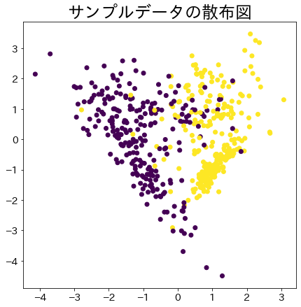
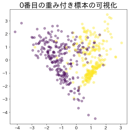
Adaboostのデータの重みの可視化
# 分類がしにくいデータに対して重みを割り当てる様子を可視化します。
 1
 2
 3
 4
 5
 6
 7
 8
 9
10
11
12
13
14
15
16
17
18
19
20
21
22
23
24
25
26
27
28
29
30
31
32
33
34
35
36
37
38
39
40
41
42
43
44
# NOTE: モデルに渡されるsample_weightを確認するために作成したモデルです
# このDummyClassifierがAdaboostのパラメタを変更することはありません
class DummyClassifier :
def __init__ ( self ):
self . model = DecisionTreeClassifier ( max_depth = 3 )
self . n_classes_ = 2
self . classes_ = [ "A" , "B" ]
self . sample_weight = None ## sample_weight
def fit ( self , X , y , sample_weight = None ):
self . sample_weight = sample_weight
self . model . fit ( X , y , sample_weight = sample_weight )
return self . model
def predict ( self , X , check_input = True ):
proba = self . model . predict ( X )
return proba
def get_params ( self , deep = False ):
return {}
def set_params ( self , deep = False ):
return {}
n_samples = 500
X_2 , y_2 = make_classification (
n_samples = n_samples ,
n_features = 2 ,
n_informative = 2 ,
n_redundant = 0 ,
n_repeated = 0 ,
random_state = 117 ,
n_clusters_per_class = 2 ,
)
plt . figure (
figsize = (
7 ,
7 ,
)
)
plt . title ( f "サンプルデータの散布図" )
plt . scatter ( X_2 [:, 0 ], X_2 [:, 1 ], c = y_2 )
plt . show ()
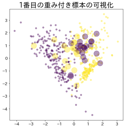
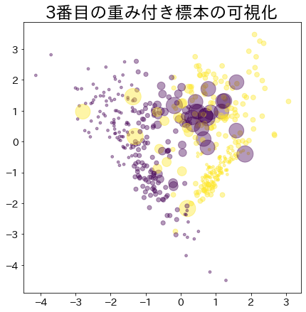
ブースティングが進んだ後の重み
# より重みがあるデータほど大きな円で表現されます。
1
2
3
4
5
6
7
8
9
10
11
12
13
14
15
16
17
18
19
20
21
22
clf = AdaBoostClassifier (
n_estimators = 4 , random_state = 0 , algorithm = "SAMME" , base_estimator = DummyClassifier ()
)
clf . fit ( X_2 , y_2 )
for i , estimators_i in enumerate ( clf . estimators_ ):
plt . figure (
figsize = (
7 ,
7 ,
)
)
plt . title ( f " { i } 番目の重み付き標本の可視化" )
plt . scatter (
X_2 [:, 0 ],
X_2 [:, 1 ],
marker = "o" ,
c = y_2 ,
alpha = 0.4 ,
s = estimators_i . sample_weight * n_samples ** 1.65 ,
)
plt . show ()
推定器数と AdaBoost
# 推定器数を増やすと AdaBoost の予測がどう改善するか確認できます。