Adaboost(回帰)

中級

2.4.4

Adaboost(回帰)

最終更新 2026-03-07 読了時間 3 分

まとめ

AdaBoost回帰（AdaBoost.R2）は予測誤差の大きいサンプルへ重みを寄せ、回帰器を段階的に改善する。
誤差分布に応じて重み更新が変わるため、外れ値の影響や誤差尺度の選択が性能に直結する。
n_estimators と learning_rate を交差検証で調整すると、過学習を抑えつつ汎化性能を高めやすい。

決定木回帰 — AdaBoost（回帰）は決定木を弱学習器として使います
Adaboost（分類） — 分類版を先に学ぶと理解がスムーズです

直感 #

AdaBoost回帰は、誤差の大きい領域を次の弱学習器に重点学習させる仕組みです。回ごとに『苦手なサンプル』へ注意を寄せることで、単体モデルでは表現しにくい非線形な誤差構造を補正できます。

数学的定式化（AdaBoost.R2） #

アルゴリズムの流れ #

$N$ 個の訓練データに対して初期重みを均等に設定します。

$$w_i^{(1)} = \frac{1}{N}, \quad i = 1, \dots, N$$

各ラウンド $t = 1, \dots, T$ で以下を繰り返します。

Step 1. 弱学習器の学習 — 重み分布 $w^{(t)}$ からブートストラップサンプリングして回帰器 $h_t(x)$ を学習する。

Step 2. 個体誤差の計算

各サンプルの正規化誤差を計算します。線形損失の場合:

$$e_i^{(t)} = \frac{|y_i - h_t(x_i)|}{\max_j |y_j - h_t(x_j)|}$$

Step 3. 加重誤差率の計算

$$\epsilon_t = \sum_{i=1}^{N} w_i^{(t)} \cdot e_i^{(t)}$$

$\epsilon_t \geq 0.5$ ならラウンドを棄却します。

Step 4. 信頼度の計算

$$\beta_t = \frac{\epsilon_t}{1 - \epsilon_t}$$

Step 5. サンプル重みの更新

$$w_i^{(t+1)} = \frac{w_i^{(t)} \cdot \beta_t^{1 - e_i^{(t)}}}{Z_t}$$

$Z_t$ は正規化定数です。誤差が小さいサンプル（$e_i \approx 0$）は $\beta_t^1$ で大きく重みを減らされ、誤差が大きいサンプル（$e_i \approx 1$）は $\beta_t^0 = 1$ で重みが維持されます。

最終予測 #

最終予測は $T$ 個の弱学習器の加重中央値です。

$$\hat{y} = \text{weighted-median}(\{h_t(x)\}_{t=1}^T, \{-\ln \beta_t\}_{t=1}^T)$$

信頼度の高い（$\beta_t$ が小さい）弱学習器ほど、中央値計算で大きな重みを持ちます。

損失関数のバリエーション #

scikit-learn の loss パラメータで個体誤差 $e_i^{(t)}$ の計算を切り替えられます:

`loss`	個体誤差 $e_i^{(t)}$
`linear`	$\frac{\|y_i - h_t(x_i)\|}{\max_j \|y_j - h_t(x_j)\|}$
`square`	$\left(\frac{\|y_i - h_t(x_i)\|}{\max_j \|y_j - h_t(x_j)\|}\right)^2$
`exponential`	$1 - \exp!\left(-\frac{\|y_i - h_t(x_i)\|}{\max_j \|y_j - h_t(x_j)\|}\right)$

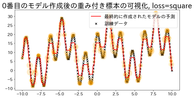
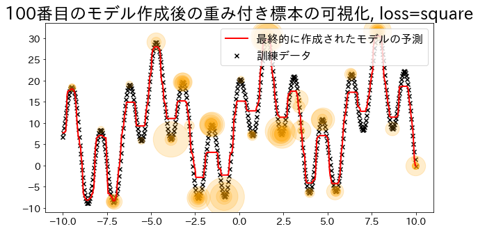
square と exponential は外れ値の影響をより強く抑えます。

詳細な解説 #

1
2
3
4
import numpy as np
import matplotlib.pyplot as plt
from sklearn.tree import DecisionTreeRegressor
from sklearn.ensemble import AdaBoostRegressor

 1
 2
 3
 4
 5
 6
 7
 8
 9
10
11
12
13
14
15
16
17
18
19
20
21
22
23
24
25
26
27
# NOTE: モデルのsample_weightを確認するために作成したモデル
class DummyRegressor:
    def __init__(self):
        self.model = DecisionTreeRegressor(max_depth=5)
        self.error_vector = None
        self.X_for_plot = None
        self.y_for_plot = None

    def fit(self, X, y):
        self.model.fit(X, y)
        y_pred = self.model.predict(X)

        # 重みは回帰の誤差を元に計算する
        # https://github.com/scikit-learn/scikit-learn/blob/main/sklearn/ensemble/_weight_boosting.py#L1130
        self.error_vector = np.abs(y_pred - y)
        self.X_for_plot = X.copy()
        self.y_for_plot = y.copy()
        return self.model

    def predict(self, X, check_input=True):
        return self.model.predict(X)

    def get_params(self, deep=False):
        return {}

    def set_params(self, deep=False):
        return {}

訓練データに回帰モデルを当てはめる #

 1
 2
 3
 4
 5
 6
 7
 8
 9
10
11
12
13
14
15
16
17
18
19
20
21
22
23
24
# 訓練データ
X = np.linspace(-10, 10, 500)[:, np.newaxis]
y = (np.sin(X).ravel() + np.cos(4 * X).ravel()) * 10 + 10 + np.linspace(-2, 2, 500)

## 回帰モデルを作成
reg = AdaBoostRegressor(
    DummyRegressor(),
    n_estimators=100,
    random_state=100,
    loss="linear",
    learning_rate=0.8,
)
reg.fit(X, y)
y_pred = reg.predict(X)

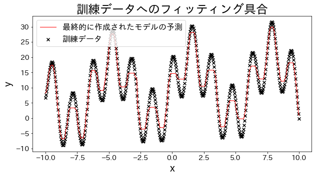
# 訓練データへのフィッティング具合を確認する
plt.figure(figsize=(10, 5))
plt.scatter(X, y, c="k", marker="x", label="訓練データ")
plt.plot(X, y_pred, c="r", label="最終的に作成されたモデルの予測", linewidth=1)
plt.xlabel("x")
plt.ylabel("y")
plt.title("訓練データへのフィッティング具合")
plt.legend()
plt.show()

png

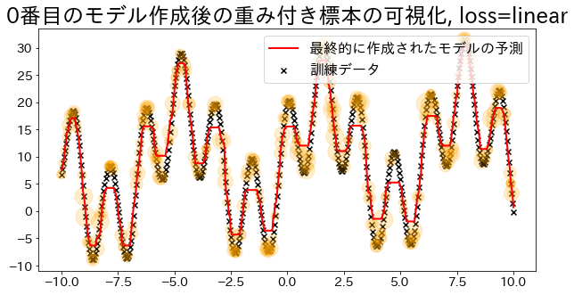
標本の重みを可視化(loss=’linear’の場合) #

Adaboostでは回帰の誤差を元い重みを決定する。’linear’ に指定した時の重みの大きさを可視化します。重みが追加されたデータは訓練時にサンプルされる確率が高くなる様子を確認します。

loss{‘linear’, ‘square’, ‘exponential’}, default=’linear’ The loss function to use when updating the weights after each boosting iteration.

sklearn.ensemble.AdaBoostRegressor

 1
 2
 3
 4
 5
 6
 7
 8
 9
10
11
12
13
14
15
16
17
18
19
20
21
22
23
24
25
26
27
28
29
30
31
32
33
34
35
36
37
38
39
40
41
42
43
44
45
46
47
48
49
50
51
52
53
54
def visualize_weight(reg, X, y, y_pred):
    """標本の重みに相当する値(サンプリングされた数)をプロットするための関数

    Parameters
    ----------
    reg : sklearn.ensemble._weight_boosting
        ブースティングモデル
    X : numpy.ndarray
        訓練データ
    y : numpy.ndarray
        教師データ
    y_pred:
        モデルの予測値
    """
    assert reg.estimators_ is not None, "len(reg.estimators_) > 0"

    for i, estimators_i in enumerate(reg.estimators_):
        if i % 100 == 0:
            # i番目のモデル作成に使用したデータに、データが何回出現するかをカウント
            weight_dict = {xi: 0 for xi in X.ravel()}
            for xi in estimators_i.X_for_plot.ravel():
                weight_dict[xi] += 1

            # 出現回数をグラフにオレンジ円でプロットする(多いほど大きい円)
            weight_x_sorted = sorted(weight_dict.items(), key=lambda x: x[0])
            weight_vec = np.array([s * 100 for xi, s in weight_x_sorted])

            # グラフをプロット
            plt.figure(figsize=(10, 5))
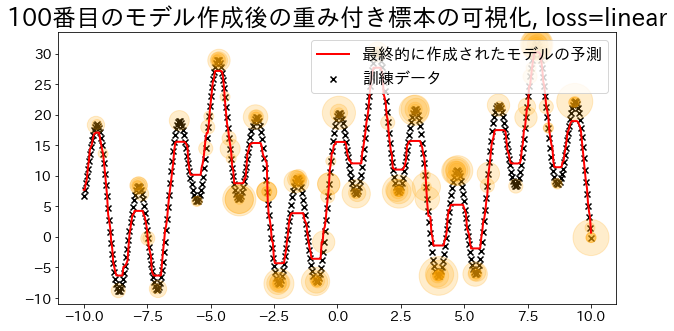
            plt.title(f"{i}番目のモデル作成後の重み付き標本の可視化, loss={reg.loss}")
            plt.scatter(X, y, c="k", marker="x", label="訓練データ")
            plt.scatter(
                estimators_i.X_for_plot,
                estimators_i.y_for_plot,
                marker="o",
                alpha=0.2,
                c="orange",
                s=weight_vec,
            )
            plt.plot(X, y_pred, c="r", label="最終的に作成されたモデルの予測", linewidth=2)
            plt.legend(loc="upper right")
            plt.show()

## loss="linear"で回帰モデルを作成
reg = AdaBoostRegressor(
    DummyRegressor(),
    n_estimators=101,
    random_state=100,
    loss="linear",
    learning_rate=1,
)
reg.fit(X, y)
y_pred = reg.predict(X)
visualize_weight(reg, X, y, y_pred)

png

png

 1
 2
 3
 4
 5
 6
 7
 8
 9
10
11
## loss="square"で回帰モデルを作成
reg = AdaBoostRegressor(
    DummyRegressor(),
    n_estimators=101,
    random_state=100,
    loss="square",
    learning_rate=1,
)
reg.fit(X, y)
y_pred = reg.predict(X)
visualize_weight(reg, X, y, y_pred)

png

png

Adaboost（分類） — 分類版
勾配ブースティング — 勾配ベースのブースティング
ランダムフォレスト — バギング系との比較

推定器数と AdaBoost 回帰 #

推定器数を増やすと予測がどう改善するか確認できます。