まとめ 勾配ブースティングは、現在モデルの残差(損失の負勾配)を次の弱学習器で順次学習していく加法モデルです。 learning_rate と n_estimators の組み合わせが、学習の進み方と過学習リスクを決める。損失関数の選択によって、外れ値への感度や最終予測の形が変化する。
直感
# 勾配ブースティングは、最初に粗い予測を作ってから「どこを外したか」を次の木で補正し続ける手法です。各ステップは小さな修正ですが、段階的に足し合わせることで複雑な関数形にも追従できるようになります。
flowchart LR
A["初期予測\n(定数)"] --> B["残差\n(負の勾配)を計算"]
B --> C["弱学習器で\n残差を学習"]
C --> D["学習率で\n加重して加算"]
D --> E{"収束?"}
E -->|No| B
E -->|Yes| F["最終予測"]
style A fill:#2563eb,color:#fff
style C fill:#1e40af,color:#fff
style F fill:#10b981,color:#fff
アルゴリズムの詳細
# 関数空間での勾配降下
# 勾配ブースティングは、任意の微分可能な損失関数\(L(y, F(\mathbf{x}))\)に対して「関数空間での勾配降下法」を行います。予測関数\(F(\mathbf{x})\)を加法的に構築します。
$$
F_m(\mathbf{x}) = F_{m-1}(\mathbf{x}) + \eta \cdot h_m(\mathbf{x})
$$ここで\(h_m\)は\(m\)番目の弱学習器(通常は浅い決定木)、\(\eta\)は学習率(縮小係数)です。
疑似残差
# 各ステップで弱学習器がフィットする対象は「疑似残差」と呼ばれる損失関数の負の勾配です。
$$
r_{im} = -\left[\frac{\partial L(y_i, F(\mathbf{x}_i))}{\partial F(\mathbf{x}_i)}\right]_{F = F_{m-1}}
$$二乗誤差\(L = \frac{1}{2}(y - F)^2\)の場合、疑似残差は単純な残差\(y_i - F_{m-1}(\mathbf{x}_i)\)と一致しますが、他の損失関数では異なります。
アルゴリズムの手順
# 初期モデルを定数に設定します: \(F_0(\mathbf{x}) = \arg\min_\gamma \sum_{i=1}^{n} L(y_i, \gamma)\) \(m = 1, \ldots, M\)について以下を繰り返します:全サンプルについて疑似残差\(r_{im}\)を計算します 決定木\(h_m\)を疑似残差\({r_{im}}\)に対してフィットします 各リーフ領域\(R_{jm}\)について最適なステップサイズを求めます: \(\gamma_{jm} = \arg\min_\gamma \sum_{x_i \in R_{jm}} L(y_i, F_{m-1}(\mathbf{x}_i) + \gamma)\) 予測を更新します: \(F_m(\mathbf{x}) = F_{m-1}(\mathbf{x}) + \eta \sum_j \gamma_{jm} \mathbf{1}(\mathbf{x} \in R_{jm})\) 最終モデル\(F_M(\mathbf{x})\)を出力します flowchart TD
A["初期モデル F₀\n(定数)"] --> B["疑似残差を計算\nrᵢ = −∂L/∂F"]
B --> C["決定木 hₘ を\n疑似残差にフィット"]
C --> D["リーフごとに\n最適ステップサイズ γⱼ"]
D --> E["更新: Fₘ = Fₘ₋₁ + η·hₘ"]
E --> F{"m = M ?"}
F -->|No| B
F -->|Yes| G["最終モデル Fₘ"]
style A fill:#2563eb,color:#fff
style C fill:#1e40af,color:#fff
style G fill:#10b981,color:#fff
損失関数と疑似残差の対応
# 損失関数 \(L(y, F)\) 疑似残差\(r_i\) 二乗誤差 \(\frac{1}{2}(y - F)^2\) \(y_i - F(\mathbf{x}_i)\) 絶対誤差 \(|y - F|\) \(\mathrm{sign}(y_i - F(\mathbf{x}_i))\) Huber \(\delta\)以下なら二乗、超えたら線形 \(\delta\)以下: \(y_i - F\)、超: \(\delta \cdot \mathrm{sign}(y_i - F)\)
縮小(Shrinkage)の理論的根拠
# 学習率\(\eta < 1\)を掛けて各木の寄与を抑えると、汎化性能が向上することが実験的に知られています。Friedman (2001) は\(\eta \approx 0.1\)を推奨しています。直感的には、各ステップで控えめに更新することで、後続の木が異なる側面から誤差を補正する余地が残り、より多様なアンサンブルが構築されます。
参考リンク
Friedman, J. H. (2001). Greedy Function Approximation: A Gradient Boosting Machine. Annals of Statistics , 29(5), 1189–1232.
詳細な解説
# 1
2
3
import numpy as np
import matplotlib.pyplot as plt
from sklearn.ensemble import GradientBoostingRegressor
訓練データに回帰モデルを当てはめる
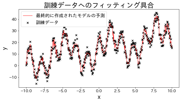
# 実験用のデータを作成します、三角関数を足し合わせた波形のデータを用意します。
1
2
3
4
5
6
7
8
9
10
11
12
13
14
15
16
17
18
19
20
21
22
23
24
25
26
27
28
29
# 訓練データ
X = np . linspace ( - 10 , 10 , 500 )[:, np . newaxis ]
noise = np . random . rand ( X . shape [ 0 ]) * 10
# 目的変数
y = (
( np . sin ( X ) . ravel () + np . cos ( 4 * X ) . ravel ()) * 10
+ 10
+ np . linspace ( - 10 , 10 , 500 )
+ noise
)
# 回帰モデルを作成
reg = GradientBoostingRegressor (
n_estimators = 50 ,
learning_rate = 0.5 ,
)
reg . fit ( X , y )
y_pred = reg . predict ( X )
# 訓練データへのフィッティング具合を確認する
plt . figure ( figsize = ( 10 , 5 ))
plt . scatter ( X , y , c = "k" , marker = "x" , label = "訓練データ" )
plt . plot ( X , y_pred , c = "r" , label = "最終的に作成されたモデルの予測" , linewidth = 1 )
plt . xlabel ( "x" )
plt . ylabel ( "y" )
plt . title ( "訓練データへのフィッティング具合" )
plt . legend ()
plt . show ()
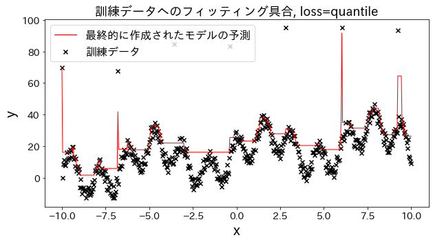
損失関数の結果への影響
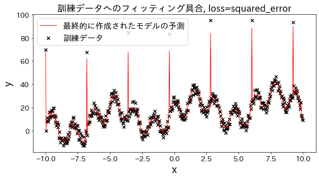
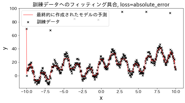
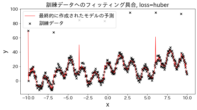
# loss を [“squared_error”, “absolute_error”, “huber”, “quantile”] と変えた場合、訓練データへのフィッティングがどのように変化するかを確認。
“absolute_error”, “huber"は二乗誤差ほど外れ値へのペナルティが大きくないので、外れ値を予測しに行かないです。
 1
 2
 3
 4
 5
 6
 7
 8
 9
10
11
12
13
14
15
16
17
18
19
20
21
22
23
24
25
26
27
28
29
30
31
32
33
34
35
36
# 訓練データ
X = np . linspace ( - 10 , 10 , 500 )[:, np . newaxis ]
# 外れ値を用意
noise = np . random . rand ( X . shape [ 0 ]) * 10
for i , ni in enumerate ( noise ):
if i % 80 == 0 :
noise [ i ] = 70 + np . random . randint ( - 10 , 10 )
# 目的変数
y = (
( np . sin ( X ) . ravel () + np . cos ( 4 * X ) . ravel ()) * 10
+ 10
+ np . linspace ( - 10 , 10 , 500 )
+ noise
)
for loss in [ "squared_error" , "absolute_error" , "huber" , "quantile" ]:
# 回帰モデルを作成
reg = GradientBoostingRegressor (
n_estimators = 50 ,
learning_rate = 0.5 ,
loss = loss ,
)
reg . fit ( X , y )
y_pred = reg . predict ( X )
# 訓練データへのフィッティング具合を確認する
plt . figure ( figsize = ( 10 , 5 ))
plt . scatter ( X , y , c = "k" , marker = "x" , label = "訓練データ" )
plt . plot ( X , y_pred , c = "r" , label = "最終的に作成されたモデルの予測" , linewidth = 1 )
plt . xlabel ( "x" )
plt . ylabel ( "y" )
plt . title ( f "訓練データへのフィッティング具合, loss= { loss } " , fontsize = 18 )
plt . legend ()
plt . show ()
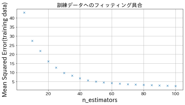
n_estimatorsの結果への影響
# ある程度 n_estimatorsを大きくすると、改善度合いは頭打ちになる様子が確認できます。
 1
 2
 3
 4
 5
 6
 7
 8
 9
10
11
12
13
14
15
16
17
18
19
20
21
22
23
24
25
26
27
28
29
30
31
32
33
34
35
from sklearn.metrics import mean_squared_error as MSE
# 訓練データ
X = np . linspace ( - 10 , 10 , 500 )[:, np . newaxis ]
noise = np . random . rand ( X . shape [ 0 ]) * 10
# 目的変数
y = (
( np . sin ( X ) . ravel () + np . cos ( 4 * X ) . ravel ()) * 10
+ 10
+ np . linspace ( - 10 , 10 , 500 )
+ noise
)
# n_estimatorsを変えてモデルを作成してみる
n_estimators_list = [( i + 1 ) * 5 for i in range ( 20 )]
mses = []
for n_estimators in n_estimators_list :
# 回帰モデルを作成
reg = GradientBoostingRegressor (
n_estimators = n_estimators ,
learning_rate = 0.3 ,
)
reg . fit ( X , y )
y_pred = reg . predict ( X )
mses . append ( MSE ( y , y_pred ))
# n_estimatorsを変えた時のmean_squared_errorをプロット
plt . figure ( figsize = ( 10 , 5 ))
plt . plot ( n_estimators_list , mses , "x" )
plt . xlabel ( "n_estimators" )
plt . ylabel ( "Mean Squared Error(training data)" )
plt . title ( f "訓練データへのフィッティング具合" , fontsize = 18 )
plt . grid ()
plt . show ()
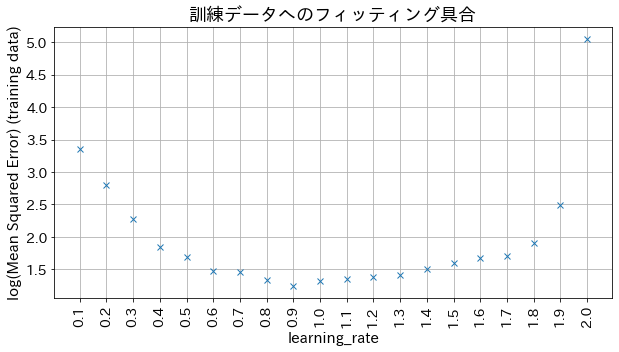
learning_rateの結果への影響
# 小さすぎると精度が良くならない、大きすぎると収束しない様子が確認できます。
 1
 2
 3
 4
 5
 6
 7
 8
 9
10
11
12
13
14
15
16
17
18
19
20
21
22
23
# n_estimatorsを変えてモデルを作成してみる
learning_rate_list = [ np . round ( 0.1 * ( i + 1 ), 1 ) for i in range ( 20 )]
mses = []
for learning_rate in learning_rate_list :
# 回帰モデルを作成
reg = GradientBoostingRegressor (
n_estimators = 30 ,
learning_rate = learning_rate ,
)
reg . fit ( X , y )
y_pred = reg . predict ( X )
mses . append ( np . log ( MSE ( y , y_pred )))
# n_estimatorsを変えた時のmean_squared_errorをプロット
plt . figure ( figsize = ( 10 , 5 ))
plt_index = [ i for i in range ( len ( learning_rate_list ))]
plt . plot ( plt_index , mses , "x" )
plt . xticks ( plt_index , learning_rate_list , rotation = 90 )
plt . xlabel ( "learning_rate" , fontsize = 15 )
plt . ylabel ( "log(Mean Squared Error) (training data)" , fontsize = 15 )
plt . title ( f "訓練データへのフィッティング具合" , fontsize = 18 )
plt . grid ()
plt . show ()
learning_rateを小さくするとn_estimatorsを大きくする必要があり、計算コストが増加します。max_depthを深くしすぎると過学習しやすくなるため、max_depth=3〜5程度から試し、early_stopping_roundsで適切な木の数を自動決定してください。
まずlearning_rate=0.1、max_depth=3で学習し、n_estimatorsをearly_stoppingで決めるのが実践的です。外れ値が多いデータではloss="huber"を試すと頑健な予測が得られます。
まとめ
# 勾配ブースティングは残差を逐次学習することで複雑な関数形に追従できるアンサンブル手法です。 learning_rateとn_estimatorsはトレードオフの関係にあり、小さい学習率ほど多くの木が必要になります。損失関数の選択(squared_error、huber、quantileなど)により外れ値への感度を制御できます。 過学習を防ぐためにmax_depthの制限とearly_stoppingの活用が重要です。 推定器数と予測曲線
# 推定器数(n_estimators)を増やすとアンサンブルの予測がどう改善するか確認できます。