まとめ ランダムフォレストは、ブートストラップ標本と特徴量のランダム部分集合を使って多数の決定木を学習し、予測を平均化・多数決する。 木ごとのばらつきを平均化することで分散を抑え、単体の決定木より汎化性能を安定させやすい。 n_estimators や max_features、木の深さの調整が、精度・計算コスト・過学習耐性のバランスを決める。
直感
# 同じデータでも、サンプリングと特徴量選択を少しずつ変えて多数の木を作ると、各木の誤差のクセが分散します。最終予測を集約すると、偶然のノイズに引っ張られた判断が打ち消され、頑健な予測になります。
flowchart LR
A["学習データ"] --> B["ブートストラップ\nサンプリング"]
B --> C["特徴量の\nランダム選択"]
C --> D["決定木を学習\n×n_estimators"]
D --> E["予測を集約\n多数決/平均"]
E --> F["最終予測"]
style A fill:#2563eb,color:#fff
style D fill:#1e40af,color:#fff
style F fill:#10b981,color:#fff
数学的定式化
# 特徴量のランダムサブセット
# ランダムフォレストはバギングに加えて、各ノード分割時に $p$ 個の特徴量から $m$ 個をランダムに選びます:
分類 : $m = \lfloor\sqrt{p}\rfloor$回帰 : $m = \lfloor p/3 \rfloor$これにより木同士の相関 $\rho$ が下がり、バギングの分散低減効果が強化されます:
$$\text{Var}(\bar{h}) = \rho \sigma^2 + \frac{1 - \rho}{B}\sigma^2$$変数重要度
# MDI(Mean Decrease in Impurity / Gini Importance) :
$$\text{MDI}(j) = \sum_{\text{tree } b} \sum_{\text{node } t \text{ splits on } j} p(t) \cdot \Delta i(t)$$$p(t)$ はノード $t$ に到達するサンプルの割合、$\Delta i(t)$ は分割による不純度の減少量です。
MDA(Mean Decrease in Accuracy / Permutation Importance) :
$$\text{MDA}(j) = \frac{1}{B}\sum_{b=1}^{B} \left[\text{Err}_{b}^{(j\text{-permuted})} - \text{Err}_{b}^{(\text{OOB})}\right]$$特徴量$j$の値をランダムに置換したときのOOB誤差増加量を測定します。MDIと比べてバイアスが少なく、推奨されることが多い手法です。
詳細な解説
# 1
2
import numpy as np
import matplotlib.pyplot as plt
ランダムフォレストを学習
# ROC-AUCについては、ROC-AUC にプロットの仕方について説明を載せています。
1
2
3
4
5
6
7
8
9
10
11
12
13
14
15
16
17
18
19
20
21
22
23
24
25
26
from sklearn.datasets import make_classification
from sklearn.ensemble import RandomForestClassifier
from sklearn.model_selection import train_test_split
from sklearn.metrics import roc_auc_score
n_features = 20
X , y = make_classification (
n_samples = 2500 ,
n_features = n_features ,
n_informative = 10 ,
n_classes = 2 ,
n_redundant = 0 ,
n_clusters_per_class = 4 ,
random_state = 777 ,
)
X_train , X_test , y_train , y_test = train_test_split (
X , y , test_size = 0.33 , random_state = 777
)
model = RandomForestClassifier (
n_estimators = 50 , max_depth = 3 , random_state = 777 , bootstrap = True , oob_score = True
)
model . fit ( X_train , y_train )
y_pred = model . predict ( X_test )
rf_score = roc_auc_score ( y_test , y_pred )
print ( f "テストデータでのROC-AUC = { rf_score } " )
テストデータでのROC-AUC = 0.814573097628059
ランダムフォレストに含まれる各木の性能を確認する
# 1
2
3
4
5
6
7
8
9
10
11
12
13
14
15
estimator_scores = []
for i in range ( 10 ):
estimator = model . estimators_ [ i ]
estimator_pred = estimator . predict ( X_test )
estimator_scores . append ( roc_auc_score ( y_test , estimator_pred ))
plt . figure ( figsize = ( 10 , 4 ))
bar_index = [ i for i in range ( len ( estimator_scores ))]
plt . bar ( bar_index , estimator_scores )
plt . bar ([ 10 ], rf_score )
plt . xticks ( bar_index + [ 10 ], bar_index + [ "RF" ])
plt . xlabel ( "木のインデックス" )
plt . ylabel ( "ROC-AUC" )
plt . show ()
特徴の重要度
# 不純度(impurity)に基づいた重要度
# 1
2
3
4
5
6
plt . figure ( figsize = ( 10 , 4 ))
feature_index = [ i for i in range ( n_features )]
plt . bar ( feature_index , model . feature_importances_ )
plt . xlabel ( "特徴のインデックス" )
plt . ylabel ( "特徴の重要度" )
plt . show ()
permutation importance
# 1
2
3
4
5
6
7
8
9
10
11
from sklearn.inspection import permutation_importance
p_imp = permutation_importance (
model , X_train , y_train , n_repeats = 10 , random_state = 77
) . importances_mean
plt . figure ( figsize = ( 10 , 4 ))
plt . bar ( feature_index , p_imp )
plt . xlabel ( "特徴のインデックス" )
plt . ylabel ( "特徴の重要度" )
plt . show ()
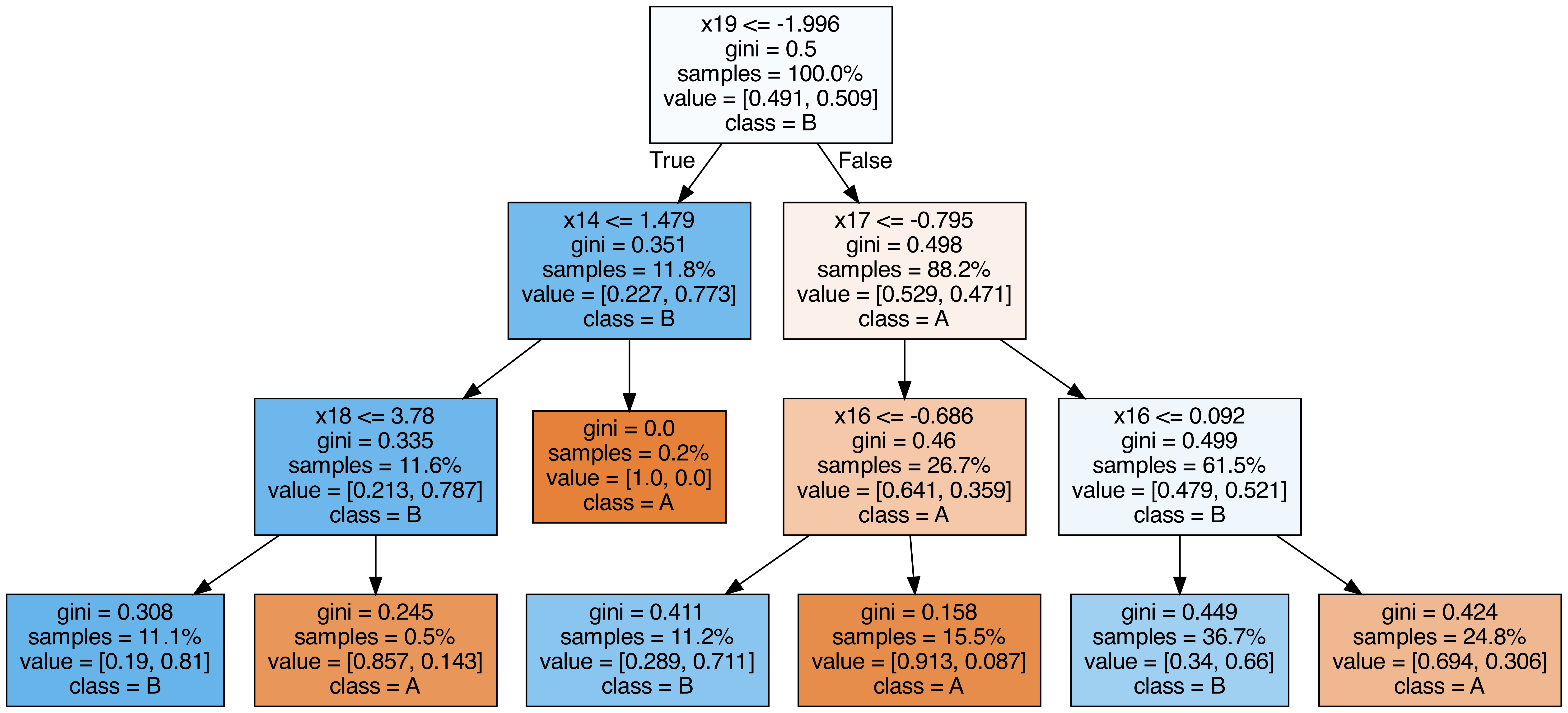
ランダムフォレストに含まれる各木を出力する
# 1
2
3
4
5
6
7
8
9
10
11
12
13
14
15
16
17
18
19
20
21
22
from sklearn.tree import export_graphviz
from subprocess import call
from IPython.display import Image
from IPython.display import display
for i in range ( 10 ):
try :
estimator = model . estimators_ [ i ]
export_graphviz (
estimator ,
out_file = f "tree { i } .dot" ,
feature_names = [ f "x { i } " for i in range ( n_features )],
class_names = [ "A" , "B" ],
proportion = True ,
filled = True ,
)
call ([ "dot" , "-Tpng" , f "tree { i } .dot" , "-o" , f "tree { i } .png" , "-Gdpi=500" ])
display ( Image ( filename = f "tree { i } .png" ))
except KeyboardInterrupt :
# TODO: jupyter bookビルド時に出力に失敗するため一時的に例外処理を挟む
pass
OOB(out-of-bag) Score
# OOBによる検証とテストデータでの検証結果が近い値を取ることが確認できます。
乱数と木の深さを変えつつ、OOBでのAccuracyとテストデータでのAccuracyを比較します。
 1
 2
 3
 4
 5
 6
 7
 8
 9
10
11
12
13
14
15
from sklearn.metrics import accuracy_score
for i in range ( 10 ):
model_i = RandomForestClassifier (
n_estimators = 50 ,
max_depth = 3 + i % 2 ,
random_state = i ,
bootstrap = True ,
oob_score = True ,
)
model_i . fit ( X_train , y_train )
y_pred = model_i . predict ( X_test )
oob_score = model_i . oob_score_
test_score = accuracy_score ( y_test , y_pred )
print ( f "OOBでの検証結果= { oob_score } テストデータでの検証結果= { test_score } " )
OOBでの検証結果=0.786865671641791 テストデータでの検証結果=0.8121212121212121
OOBでの検証結果=0.8101492537313433 テストデータでの検証結果=0.8363636363636363
OOBでの検証結果=0.7886567164179105 テストデータでの検証結果=0.8024242424242424
OOBでの検証結果=0.8161194029850747 テストデータでの検証結果=0.8315151515151515
OOBでの検証結果=0.7910447761194029 テストデータでの検証結果=0.8072727272727273
OOBでの検証結果=0.8101492537313433 テストデータでの検証結果=0.833939393939394
OOBでの検証結果=0.7814925373134328 テストデータでの検証結果=0.8133333333333334
OOBでの検証結果=0.8059701492537313 テストデータでの検証結果=0.833939393939394
OOBでの検証結果=0.7832835820895523 テストデータでの検証結果=0.7951515151515152
OOBでの検証結果=0.8083582089552239 テストデータでの検証結果=0.8387878787878787
不純度ベースの特徴量重要度は、カーディナリティの高い特徴量(カテゴリ数が多い変数や連続値)を過大評価する傾向があります。正確な重要度を得るにはpermutation_importanceを併用してください。
n_estimatorsは大きくしても過学習しにくいため、計算リソースが許す限り増やすのが基本です。oob_score=Trueを設定するとホールドアウトなしで汎化性能を推定でき、交差検証の代わりに使えます。
まとめ
# ランダムフォレストはブートストラップサンプリングと特徴量のランダム選択で多数の決定木を学習し、集約することで汎化性能を高めます。 n_estimatorsを増やしても過学習しにくい性質があり、計算コストとのトレードオフで調整します。特徴量重要度は不純度ベースとPermutation Importanceの2種類があり、後者のほうがバイアスが少ないです。 OOBスコアを活用すると、交差検証なしで汎化性能を効率的に推定できます。