スタッキング

上級

2.4.2

スタッキング

最終更新 2026-03-07 読了時間 3 分

まとめ

スタッキングは、複数の一次モデルの予測を入力として、二次モデル（メタモデル）が最終予測を学習する手法である。
性質の異なるモデルを組み合わせることで、単一モデルでは拾い切れないパターンを補完できる。
リークを防ぐために out-of-fold 予測でメタ特徴を作る設計が、実運用での性能を左右する。

交差検証 — スタッキングは Out-of-Fold 予測を使うため CV の理解が必要です
複数の分類器/回帰モデルの基本（ロジスティック回帰・決定木・SVM など）

直感 #

スタッキングは「モデルを重ねる」発想です。まず複数モデルに同じ問題を解かせ、次にそれぞれの予測の得意・不得意を見て、最終モデルが重み付けして結論を出します。重要なのは、学習時に見た答えを二段目へ漏らさない分割設計です。

数学的定式化 #

2層アーキテクチャ #

スタッキングは 2 層のモデル構造です:

Level-0（ベース学習器）: $K$ 個の多様なモデル $h_1, h_2, \dots, h_K$ を訓練データで学習する。

Level-1（メタ学習器）: ベース学習器の予測を特徴量として受け取り、最終予測を行うモデル $g$ を学習する。

$$\hat{y} = g\!\left(h_1(x),\; h_2(x),\; \dots,\; h_K(x)\right)$$

Out-of-Fold 予測（リーク防止） #

メタ学習器の訓練データを作る際、ベース学習器が自身の訓練データをそのまま予測するとリーク（情報漏洩）が起きます。これを防ぐために Out-of-Fold (OOF) 予測を使います:

訓練データを $J$ 個の Fold に分割
Fold $j$ を除いた残りでベース学習器 $h_k$ を学習
Fold $j$ のデータを予測し、メタ特徴 $z_{ij}^{(k)}$ とする
全 Fold の予測を結合して、メタ特徴行列 $Z \in \mathbb{R}^{N \times K}$ を構成

$$Z = \begin{pmatrix} z_{11} & z_{12} & \cdots & z_{1K} \\ z_{21} & z_{22} & \cdots & z_{2K} \\ \vdots & \vdots & \ddots & \vdots \\ z_{N1} & z_{N2} & \cdots & z_{NK} \end{pmatrix}$$

メタ学習器はこの $Z$ と元のラベル $y$ を使って学習します: $g: Z \to y$。

flowchart TD A["訓練データ"] --> B["K-Fold 分割"] B --> C1["Fold 1 を除いて\nベース学習器を学習"] B --> C2["Fold 2 を除いて\nベース学習器を学習"] B --> C3["Fold J を除いて\nベース学習器を学習"] C1 --> D1["Fold 1 の\nOOF 予測"] C2 --> D2["Fold 2 の\nOOF 予測"] C3 --> D3["Fold J の\nOOF 予測"] D1 --> E["メタ特徴行列 Z"] D2 --> E D3 --> E E --> F["メタ学習器 g を学習"] F --> G["最終予測"] style A fill:#2563eb,color:#fff style E fill:#1e40af,color:#fff style G fill:#10b981,color:#fff

詳細な解説 #

 1
 2
 3
 4
 5
 6
 7
 8
 9
10
import matplotlib.pyplot as plt

from sklearn.datasets import make_classification
from sklearn.tree import DecisionTreeClassifier
from sklearn.ensemble import RandomForestClassifier
from sklearn.ensemble import StackingClassifier
from sklearn.model_selection import train_test_split
from sklearn.metrics import roc_auc_score
from sklearn.tree import export_graphviz
from subprocess import call

実験用のデータを作成 #

 1
 2
 3
 4
 5
 6
 7
 8
 9
10
11
12
13
14
# 特徴が20あるデータを作成
n_features = 20
X, y = make_classification(
    n_samples=2500,
    n_features=n_features,
    n_informative=10,
    n_classes=2,
    n_redundant=0,
    n_clusters_per_class=4,
    random_state=777,
)
X_train, X_test, y_train, y_test = train_test_split(
    X, y, test_size=0.33, random_state=777
)

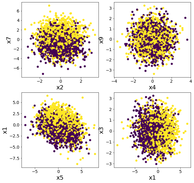
データを複数の特徴に関してプロットしてみる #

単純なルールでは分類できなさそうであることを確認する。

 1
 2
 3
 4
 5
 6
 7
 8
 9
10
11
12
13
14
15
16
17
18
plt.figure(figsize=(10, 10))
plt.subplot(2, 2, 1)
plt.scatter(X[:, 2], X[:, 7], c=y)
plt.xlabel("x2")
plt.ylabel("x7")
plt.subplot(2, 2, 2)
plt.scatter(X[:, 4], X[:, 9], c=y)
plt.xlabel("x4")
plt.ylabel("x9")
plt.subplot(2, 2, 3)
plt.scatter(X[:, 5], X[:, 1], c=y)
plt.xlabel("x5")
plt.ylabel("x1")
plt.subplot(2, 2, 4)
plt.scatter(X[:, 1], X[:, 3], c=y)
plt.xlabel("x1")
plt.ylabel("x3")
plt.show()

png

スタッキングとランダムフォレストの比較 #

ランダムフォレストで分類してみた場合 #

1
2
3
4
5
model = RandomForestClassifier(n_estimators=50, max_depth=5, random_state=777)
model.fit(X_train, y_train)
y_pred = model.predict(X_test)
rf_score = roc_auc_score(y_test, y_pred)
print(f"ROC-AUC = {rf_score}")

ROC-AUC = 0.855797033310609

複数の木でスタッキングした場合 #

DecisionTreeClassifierのみでスタッキングしても精度があまり向上しないことが確認できる。

sklearn.ensemble.StackingClassifier

 1
 2
 3
 4
 5
 6
 7
 8
 9
10
11
12
13
14
15
16
17
18
19
20
# スタッキング前段に使用するモデル
estimators = [
    ("dt1", DecisionTreeClassifier(max_depth=3, random_state=777)),
    ("dt2", DecisionTreeClassifier(max_depth=4, random_state=777)),
    ("dt3", DecisionTreeClassifier(max_depth=5, random_state=777)),
    ("dt4", DecisionTreeClassifier(max_depth=6, random_state=777)),
]
# スタッキングに含まれるモデル数
n_estimators = len(estimators)
# スタッキング後段に使用するモデル
final_estimator = DecisionTreeClassifier(max_depth=3, random_state=777)
# スタッキングモデルを作成し訓練する
clf = StackingClassifier(estimators=estimators, final_estimator=final_estimator)
clf.fit(X_train, y_train)
# テストデータで評価する
y_pred = clf.predict(X_test)
clf_score = roc_auc_score(y_test, y_pred)

print("ROC-AUC")
print(f"決定木のスタッキング＝{clf_score}, ランダムフォレスト＝{rf_score}")

ROC-AUC
決定木のスタッキング＝0.7359716965608031, ランダムフォレスト＝0.855797033310609

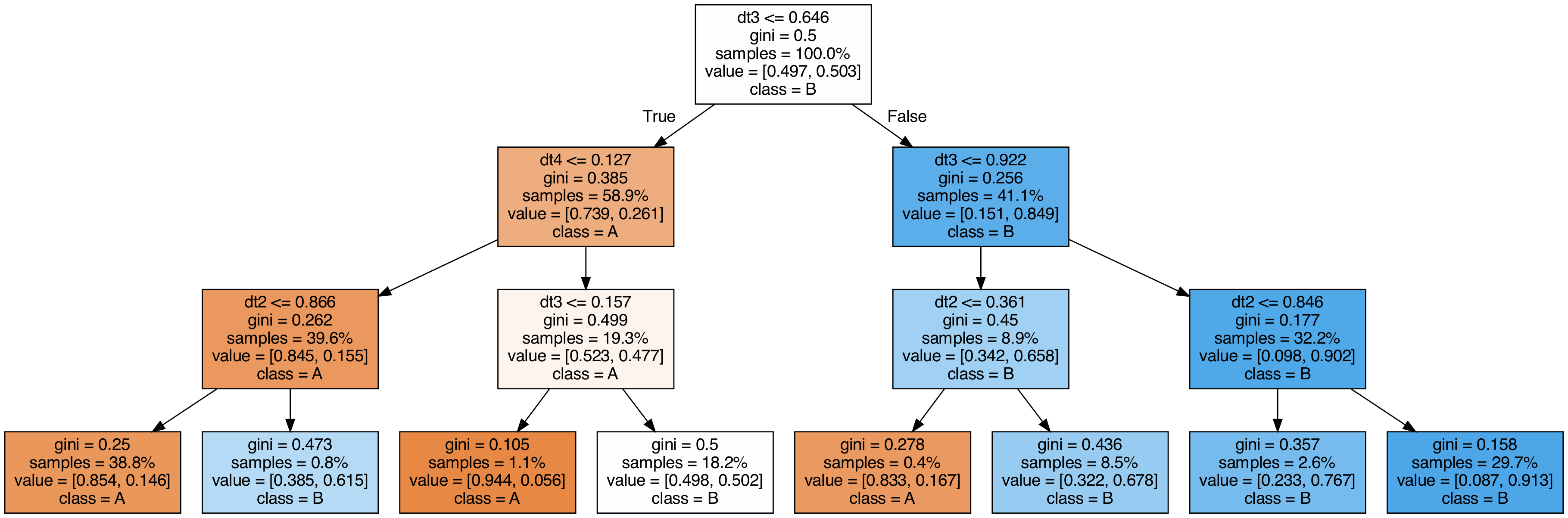
スタッキングに使用した木を可視化してみる #

 1
 2
 3
 4
 5
 6
 7
 8
 9
10
11
12
13
14
15
16
17
18
19
20
export_graphviz(
    clf.final_estimator_,
    out_file="tree_final_estimator.dot",
    class_names=["A", "B"],
    feature_names=[e[0] for e in estimators],
    proportion=True,
    filled=True,
)

call(
    [
        "dot",
        "-Tpng",
        "tree_final_estimator.dot",
        "-o",
        f"tree_final_estimator.png",
        "-Gdpi=200",
    ]
)
display(Image(filename="tree_final_estimator.png"))

png

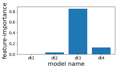
スタッキングで使用した木の特徴重要度を見る #

スタッキングしたものの、結局4番目の木しかほとんど予測に利用されていないことが分かる。

1
2
3
4
5
6
7
plt.figure(figsize=(6, 3))
plot_index = [i for i in range(n_estimators)]
plt.bar(plot_index, clf.final_estimator_.feature_importances_)
plt.xticks(plot_index, [e[0] for e in estimators])
plt.xlabel("model name")
plt.ylabel("feature-importance")
plt.show()

png

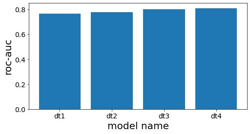
スタッキング前段の各木の性能を確認する #

 1
 2
 3
 4
 5
 6
 7
 8
 9
10
11
12
13
14
15
16
17
18
19
20
# スタッキング前段の木の精度を計測する
scores = []
for clf_estim in clf.estimators_:
    print("====")
    y_pred = clf_estim.predict(X_test)
    scr = roc_auc_score(y_test, y_pred)
    scores.append(scr)
    print(clf_estim)
    print(scr)

n_estimators = len(estimators)
plot_index = [i for i in range(n_estimators)]

# グラフ作成
plt.figure(figsize=(8, 4))
plt.bar(plot_index, scores)
plt.xticks(plot_index, [e[0] for e in estimators])
plt.xlabel("model name")
plt.ylabel("roc-auc")
plt.show()

====
DecisionTreeClassifier(max_depth=3, random_state=777)
0.7660117774277722
====
DecisionTreeClassifier(max_depth=4, random_state=777)
0.7744128916993818
====
DecisionTreeClassifier(max_depth=5, random_state=777)
0.8000158677919086
====
DecisionTreeClassifier(max_depth=6, random_state=777)
0.8084639977432473

png

・Stacked Generalization (Stacking)
・MLWave/Kaggle-Ensemble-Guide

バギング — 並列アンサンブル
勾配ブースティング — 逐次アンサンブル
ランダムフォレスト — ベース学習器の候補