XGBoost

中級

2.4.9

XGBoost

最終更新 2020-05-20 読了時間 4 分

まとめ

XGBoost（eXtreme Gradient Boosting）は正則化項を目的関数に組み込み、過学習を抑えながら高精度を実現する勾配ブースティング実装。
欠損値の自動処理、列サンプリング、ヒストグラム近似など、大規模データ向けの高速化手法を備える。
learning_rate・max_depth・n_estimators・reg_alpha/reg_lambdaが主なチューニング対象。

勾配ブースティング — XGBoost は勾配ブースティングの高速・正則化実装です

直感 #

勾配ブースティングは弱い木を順番に足していく手法だが、木を増やしすぎると過学習しやすい。XGBoostは目的関数にL1/L2正則化を加えて木の複雑さにペナルティを課すことで、この問題を軽減する。さらに、欠損値を自動で最適な方向に割り振る仕組みや、列サンプリングによるランダム性の導入など、実務で便利な機能が多い。

flowchart LR A["学習データ"] --> B["初期予測\n(定数)"] B --> C["残差を計算"] C --> D["決定木で残差を学習\n+ L1/L2正則化"] D --> E["学習率ηで\n予測に加算"] E --> F{"収束？\nn_estimators?"} F -->|No| C F -->|Yes| G["最終予測"] style A fill:#2563eb,color:#fff style D fill:#1e40af,color:#fff style G fill:#10b981,color:#fff

アルゴリズムの詳細 #

正則化付き目的関数 #

XGBoostは$t$番目の木を追加する際、以下の目的関数を最小化します。

$$ \mathcal{L}^{(t)} = \sum_{i=1}^{n} l\bigl(y_i,\; \hat{y}_i^{(t-1)} + f_t(\mathbf{x}_i)\bigr) + \Omega(f_t) $$

ここで$l$は微分可能な損失関数、$f_t$は新たに追加する木、$\Omega$は木の複雑さに対する正則化項です。

$$ \Omega(f) = \gamma\, T + \frac{1}{2}\lambda \sum_{j=1}^{T} w_j^2 $$

$T$は葉の数、$w_j$は各葉の重み、$\gamma$は葉の数に対するペナルティ、$\lambda$はL2正則化の強さです。

2次テイラー展開による近似 #

損失関数を$f_t(\mathbf{x}_i)$について2次までテイラー展開すると、定数項を除いて以下の近似が得られます。

$$ \tilde{\mathcal{L}}^{(t)} \approx \sum_{i=1}^{n} \left[ g_i\, f_t(\mathbf{x}_i) + \frac{1}{2} h_i\, f_t(\mathbf{x}_i)^2 \right] + \Omega(f_t) $$$$ g_i = \frac{\partial\, l(y_i, \hat{y}^{(t-1)})}{\partial\, \hat{y}^{(t-1)}}, \qquad h_i = \frac{\partial^2 l(y_i, \hat{y}^{(t-1)})}{\partial\, (\hat{y}^{(t-1)})^2} $$

$g_i$は1次勾配、$h_i$は2次勾配（ヘッセ行列の対角成分）です。2次情報を使うことで、通常の勾配ブースティング（1次のみ）より効率的な最適化が可能になります。

最適な葉の重みと目的関数値 #

葉$j$に属するサンプルの集合を$I_j$とし、$G_j = \sum_{i \in I_j} g_i$、$H_j = \sum_{i \in I_j} h_i$とすると、最適な葉の重みは以下で求まります。

$$ w_j^* = -\frac{G_j}{H_j + \lambda} $$

このとき目的関数の最小値は

$$ \tilde{\mathcal{L}}^* = -\frac{1}{2} \sum_{j=1}^{T} \frac{G_j^2}{H_j + \lambda} + \gamma\, T $$

です。この値が小さいほど、その木構造が損失をよく減らすことを意味します。

分割ゲイン #

ノードを左右に分割するかどうかは、分割前後の目的関数の差（ゲイン）で判断します。

$$ \text{Gain} = \frac{1}{2}\left[\frac{G_L^2}{H_L + \lambda} + \frac{G_R^2}{H_R + \lambda} - \frac{(G_L + G_R)^2}{H_L + H_R + \lambda}\right] - \gamma $$

$G_L, H_L$は左の子ノード、$G_R, H_R$は右の子ノードの勾配統計量です。Gainが正のときのみ分割を採用し、$\gamma$が大きいほど分割が抑制されます。

flowchart TD A["損失関数 l(y, ŷ)"] --> B["1次勾配 gᵢ\n2次勾配 hᵢ を計算"] B --> C["候補分割点ごとに\nGain を計算"] C --> D{"Gain > γ ?"} D -->|Yes| E["分割を採用\nG_L,H_L / G_R,H_R に分配"] D -->|No| F["葉として確定\nw* = −G/(H+λ)"] E --> C style A fill:#2563eb,color:#fff style C fill:#1e40af,color:#fff style F fill:#10b981,color:#fff

高速化技法 #

スパース対応分割: 欠損値を持つサンプルを左右どちらに送るかを自動的に学習し、欠損値の最適な処理方向を決定します
列サンプリング: ランダムフォレストのアイデアを取り入れ、各木または各分割で使う特徴量のサブセットをランダムに選択します。過学習の抑制と計算速度の向上を両立します
加重量子化スケッチ: 大規模データでは全候補点を列挙できないため、重み付き量子化スケッチで近似的な分割候補を効率的に見つけます

参考リンク

Chen, T., & Guestrin, C. (2016). XGBoost: A Scalable Tree Boosting System. Proceedings of the 22nd ACM SIGKDD International Conference on Knowledge Discovery and Data Mining, 785–794.

詳細な解説 #

XGBoost Documentation

ライブラリと実験データ #

1
2
3
4
5
6
import numpy as np
import matplotlib.pyplot as plt
from sklearn.datasets import make_classification
from sklearn.model_selection import train_test_split
from sklearn.metrics import roc_auc_score
from xgboost import XGBClassifier

二値分類用の合成データを作成し、学習・テストに分割します。

1
2
3
4
5
6
7
X, y = make_classification(
    n_samples=1000, n_features=20, n_informative=10,
    n_redundant=5, random_state=42
)
X_train, X_test, y_train, y_test = train_test_split(
    X, y, test_size=0.3, random_state=42
)

基本的な学習と評価 #

 1
 2
 3
 4
 5
 6
 7
 8
 9
10
model = XGBClassifier(
    n_estimators=100,
    max_depth=5,
    learning_rate=0.1,
    random_state=42,
    eval_metric="logloss",
)
model.fit(X_train, y_train)
y_prob = model.predict_proba(X_test)[:, 1]
print(f"ROC-AUC: {roc_auc_score(y_test, y_prob):.4f}")

learning_rateの影響 #

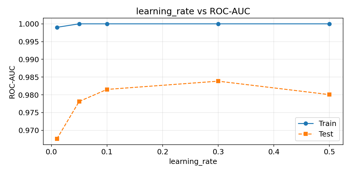
学習率を変えると、各ステップで加える木の寄与度が変わります。小さいほど精度は上がりやすいが、必要なステップ数が増えます。学習データとテストデータの両方でスコアを確認すると、過学習の兆候も把握できます。

 1
 2
 3
 4
 5
 6
 7
 8
 9
10
11
12
13
14
15
16
17
18
19
20
21
rates = [0.01, 0.05, 0.1, 0.3, 0.5]
train_scores, test_scores = [], []
for lr in rates:
    m = XGBClassifier(
        n_estimators=200, max_depth=5,
        learning_rate=lr, random_state=42,
        eval_metric="logloss",
    )
    m.fit(X_train, y_train)
    train_scores.append(roc_auc_score(y_train, m.predict_proba(X_train)[:, 1]))
    test_scores.append(roc_auc_score(y_test, m.predict_proba(X_test)[:, 1]))

plt.figure(figsize=(8, 4))
plt.plot(rates, train_scores, "o-", label="Train")
plt.plot(rates, test_scores, "s--", label="Test")
plt.xlabel("learning_rate")
plt.ylabel("ROC-AUC")
plt.title("learning_rate vs ROC-AUC")
plt.legend()
plt.grid(True, alpha=0.3)
plt.show()

learning_rateとROC-AUCの関係

max_depthの影響 #

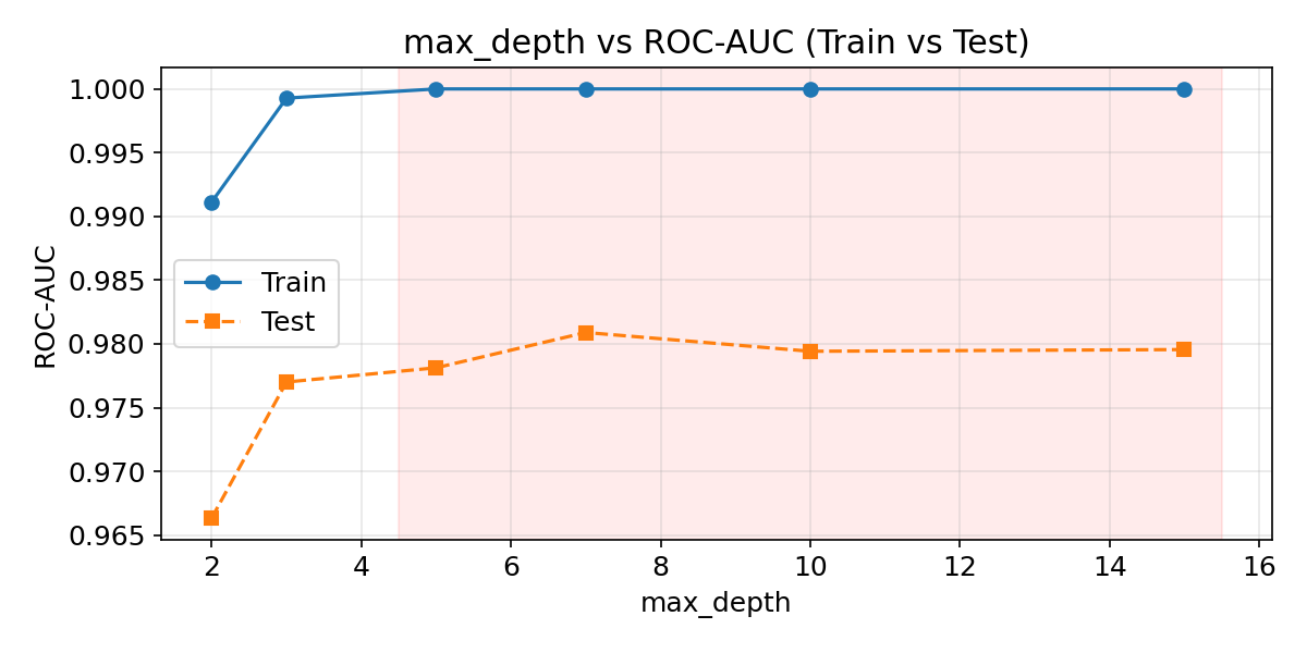
木の深さを増やすと表現力は上がるが、過学習のリスクも高まります。TrainとTestのスコア差が開くほど過学習が進んでいることを示します。

 1
 2
 3
 4
 5
 6
 7
 8
 9
10
11
12
13
14
15
16
17
18
19
20
21
depths = [2, 3, 5, 7, 10, 15]
train_scores, test_scores = [], []
for d in depths:
    m = XGBClassifier(
        n_estimators=100, max_depth=d,
        learning_rate=0.1, random_state=42,
        eval_metric="logloss",
    )
    m.fit(X_train, y_train)
    train_scores.append(roc_auc_score(y_train, m.predict_proba(X_train)[:, 1]))
    test_scores.append(roc_auc_score(y_test, m.predict_proba(X_test)[:, 1]))

plt.figure(figsize=(8, 4))
plt.plot(depths, train_scores, "o-", label="Train")
plt.plot(depths, test_scores, "s--", label="Test")
plt.xlabel("max_depth")
plt.ylabel("ROC-AUC")
plt.title("max_depth vs ROC-AUC (Train vs Test)")
plt.legend()
plt.grid(True, alpha=0.3)
plt.show()

max_depthとROC-AUCの関係（Train vs Test）

正則化パラメーターの影響 #

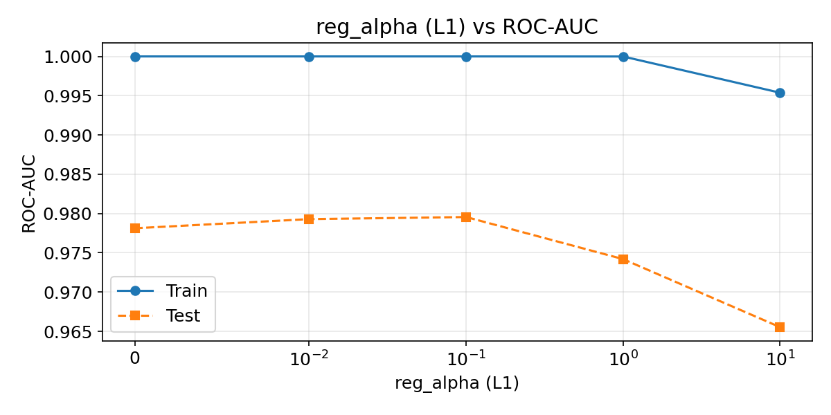
reg_alpha（L1）とreg_lambda（L2）で木の葉の重みにペナルティを与え、過学習を抑制します。

 1
 2
 3
 4
 5
 6
 7
 8
 9
10
11
12
13
14
15
16
17
18
19
20
21
22
alphas = [0, 0.01, 0.1, 1.0, 10.0]
train_scores, test_scores = [], []
for a in alphas:
    m = XGBClassifier(
        n_estimators=100, max_depth=5,
        learning_rate=0.1, reg_alpha=a,
        random_state=42, eval_metric="logloss",
    )
    m.fit(X_train, y_train)
    train_scores.append(roc_auc_score(y_train, m.predict_proba(X_train)[:, 1]))
    test_scores.append(roc_auc_score(y_test, m.predict_proba(X_test)[:, 1]))

plt.figure(figsize=(8, 4))
plt.plot(alphas, train_scores, "o-", label="Train")
plt.plot(alphas, test_scores, "s--", label="Test")
plt.xscale("symlog", linthresh=0.01)
plt.xlabel("reg_alpha (L1)")
plt.ylabel("ROC-AUC")
plt.title("reg_alpha (L1) vs ROC-AUC")
plt.legend()
plt.grid(True, alpha=0.3)
plt.show()

L1正則化とROC-AUCの関係

特徴量の重要度 #

 1
 2
 3
 4
 5
 6
 7
 8
 9
10
importances = model.feature_importances_
indices = np.argsort(importances)[::-1]

plt.figure(figsize=(10, 5))
plt.bar(range(len(importances)), importances[indices], color="#2563eb", alpha=0.8)
plt.xlabel("Feature Index")
plt.ylabel("Importance (gain)")
plt.title("XGBoost Feature Importance")
plt.xticks(range(len(importances)), [f"f{i}" for i in indices], fontsize=9)
plt.show()

XGBoost特徴量重要度

max_depthを大きくしすぎると、学習データへの過学習が急速に進みます。上のグラフでTrainスコアが1.0に近づく一方でTestスコアが下がる現象が確認できます。まずはmax_depth=3〜6の範囲で試し、early_stopping_roundsを併用して不要な木の追加を防いでください。

チューニングの優先順位は learning_rate → max_depth → n_estimators → reg_alpha/reg_lambda の順が効率的です。learning_rateを小さくしたらn_estimatorsを増やす、という組み合わせで調整してください。GridSearchCVやOptunaを使うと探索が自動化できます。

まとめ #

XGBoostは目的関数にL1/L2正則化を組み込むことで、勾配ブースティングの過学習を抑えながら高精度を実現します。
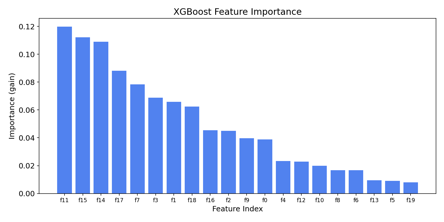
learning_rateを小さくすると精度は上がりやすいですが、必要なn_estimatorsが増えるため、両者をセットで調整します。
max_depthはTrainとTestのスコア乖離を確認しながら設定し、過学習の兆候が見えたら正則化パラメーターで抑制します。
特徴量重要度を可視化することで、モデルがどの変数に依存しているかを把握し、特徴量選択や解釈に活用できます。

Gradient Boosting（回帰） — 勾配ブースティングの基礎
LightGBM — ヒストグラム近似に特化した高速実装
CatBoost — カテゴリ変数に強い勾配ブースティング
SHAP — モデルの予測を特徴量ごとに分解して解釈
PDP / ICE — 特徴量と予測の関係を可視化

推定器数と XGBoost #

推定器数を増やすと XGBoost の予測がどう改善するか確認できます。