  1
  2
  3
  4
  5
  6
  7
  8
  9
 10
 11
 12
 13
 14
 15
 16
 17
 18
 19
 20
 21
 22
 23
 24
 25
 26
 27
 28
 29
 30
 31
 32
 33
 34
 35
 36
 37
 38
 39
 40
 41
 42
 43
 44
 45
 46
 47
 48
 49
 50
 51
 52
 53
 54
 55
 56
 57
 58
 59
 60
 61
 62
 63
 64
 65
 66
 67
 68
 69
 70
 71
 72
 73
 74
 75
 76
 77
 78
 79
 80
 81
 82
 83
 84
 85
 86
 87
 88
 89
 90
 91
 92
 93
 94
 95
 96
 97
 98
 99
100
101
102
103
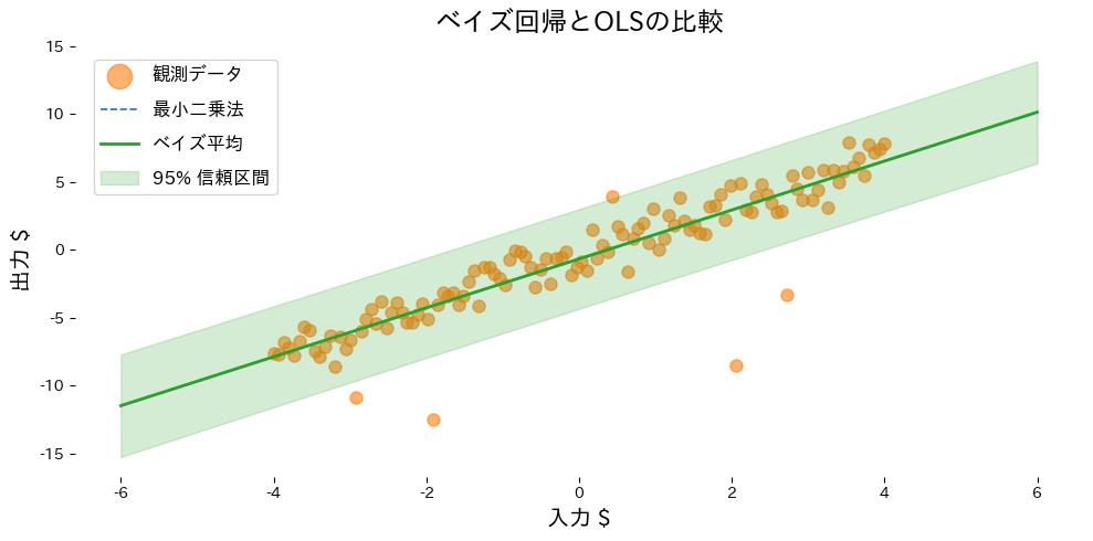
| from __future__ import annotations
import matplotlib.pyplot as plt
import numpy as np
from sklearn.linear_model import BayesianRidge, LinearRegression
from sklearn.metrics import mean_squared_error
def run_bayesian_linear_demo(
n_samples: int = 120,
noise_scale: float = 1.0,
outlier_count: int = 6,
outlier_scale: float = 8.0,
label_observations: str = "observations",
label_ols: str = "OLS",
label_bayes: str = "Bayesian mean",
label_interval: str = "95% CI",
xlabel: str = "input $",
ylabel: str = "output $",
title: str | None = None,
) -> dict[str, float]:
"""Fit OLS and Bayesian ridge to noisy data with outliers, plotting results.
Args:
n_samples: Number of evenly spaced sample points.
noise_scale: Standard deviation of Gaussian noise added to the base line.
outlier_count: Number of indices to perturb strongly.
outlier_scale: Standard deviation for the outlier noise.
label_observations: Legend label for observations.
label_ols: Label for the ordinary least squares line.
label_bayes: Label for the Bayesian posterior mean line.
label_interval: Label for the confidence interval band.
xlabel: X-axis label.
ylabel: Y-axis label.
title: Optional plot title.
Returns:
Dictionary containing MSEs and coefficients statistics.
"""
rng = np.random.default_rng(seed=0)
x_values: np.ndarray = np.linspace(-4.0, 4.0, n_samples, dtype=float)
y_clean: np.ndarray = 1.8 * x_values - 0.5
y_noisy: np.ndarray = y_clean + rng.normal(scale=noise_scale, size=x_values.shape)
outlier_idx = rng.choice(n_samples, size=outlier_count, replace=False)
y_noisy[outlier_idx] += rng.normal(scale=outlier_scale, size=outlier_idx.shape)
X: np.ndarray = x_values[:, np.newaxis]
ols = LinearRegression()
ols.fit(X, y_noisy)
bayes = BayesianRidge(compute_score=True)
bayes.fit(X, y_noisy)
X_grid: np.ndarray = np.linspace(-6.0, 6.0, 200, dtype=float)[:, np.newaxis]
ols_mean: np.ndarray = ols.predict(X_grid)
bayes_mean, bayes_std = bayes.predict(X_grid, return_std=True)
metrics = {
"ols_mse": float(mean_squared_error(y_noisy, ols.predict(X))),
"bayes_mse": float(mean_squared_error(y_noisy, bayes.predict(X))),
"coef_mean": float(bayes.coef_[0]),
"coef_std": float(np.sqrt(bayes.sigma_[0, 0])),
}
upper = bayes_mean + 1.96 * bayes_std
lower = bayes_mean - 1.96 * bayes_std
fig, ax = plt.subplots(figsize=(10, 5))
ax.scatter(X, y_noisy, color="#ff7f0e", alpha=0.6, label=label_observations)
ax.plot(X_grid, ols_mean, color="#1f77b4", linestyle="--", label=label_ols)
ax.plot(X_grid, bayes_mean, color="#2ca02c", linewidth=2, label=label_bayes)
ax.fill_between(
X_grid.ravel(),
lower,
upper,
color="#2ca02c",
alpha=0.2,
label=label_interval,
)
ax.set_xlabel(xlabel)
ax.set_ylabel(ylabel)
if title:
ax.set_title(title)
ax.legend()
fig.tight_layout()
plt.show()
return metrics
metrics = run_bayesian_linear_demo(
label_observations="観測データ",
label_ols="最小二乗法",
label_bayes="ベイズ平均",
label_interval="95% 信頼区間",
xlabel="入力 $",
ylabel="出力 $",
title="ベイズ回帰とOLSの比較",
)
print(f"OLSのMSE: {metrics['ols_mse']:.3f}")
print(f"ベイズ回帰のMSE: {metrics['bayes_mse']:.3f}")
print(f"係数の事後平均: {metrics['coef_mean']:.3f}")
print(f"係数の事後標準偏差: {metrics['coef_std']:.3f}")
|