【ベンチマーク】非線形関係の回帰

 1
 2
 3
 4
 5
 6
 7
 8
 9
10
11
12
13
14
15
16
17
18
19
20
21
22
23
24
25
26
27
28
29
30
31
32
33
34
35
36
37

import numpy as np
import pandas as pd
import matplotlib.pyplot as plt

rng = np.random.default_rng(42)
n = 500

X = rng.normal(0, 1, size=(n, 5))
y = np.sin(X[:, 0]) + X[:, 1]**2 + np.log(np.abs(X[:, 2]) + 1) + rng.normal(0, 0.3, n)
feature_names = ["x₁", "x₂", "x₃", "x₄(noise)", "x₅(noise)"]

fig, axes = plt.subplots(1, 3, figsize=(15, 4))

# 各特徴量とyの関係
for i, (ax, fname, color) in enumerate(zip(axes, ["x₁ → sin(x₁)", "x₂ → x₂²", "x₃ → log(|x₃|+1)"],
                                            ["#2563eb", "#10b981", "#f97316"])):
    ax.scatter(X[:, i], y, alpha=0.3, s=10, color=color)

    # 真の関数を重ねる
    x_sort = np.sort(X[:, i])
    if i == 0:
        y_true = np.sin(x_sort) + 1.0  # 他の項の期待値を加算
    elif i == 1:
        y_true = x_sort**2 + 0.5
    else:
        y_true = np.log(np.abs(x_sort) + 1) + 1.0

    ax.plot(x_sort, y_true, color="#ef4444", linewidth=2, label="真の関数形")
    ax.set_title(fname)
    ax.set_xlabel(feature_names[i])
    ax.set_ylabel("y")
    ax.legend(fontsize=8)
    ax.grid(alpha=0.2)

fig.suptitle("非線形データの構造", fontsize=13)
fig.tight_layout()
plt.show()

 1
 2
 3
 4
 5
 6
 7
 8
 9
10
11
12
13
14
15
16
17
18
19
20
21
22
23
24
25
26
27
28
29
30
31
32
33
34
35
36
37
38
39
40
41
42
43
44
45
46
47
48
49
50
51
52
53
54
55
56
57
58
59
60
61
62
63
64
65
66
67
68
69
70
71
72
73
74
75
76
77
78
79
80
81
82
83
84
85

from sklearn.model_selection import cross_val_score, KFold
from sklearn.linear_model import LinearRegression, Ridge
from sklearn.svm import SVR
from sklearn.neighbors import KNeighborsRegressor
from sklearn.ensemble import RandomForestRegressor, GradientBoostingRegressor
from sklearn.preprocessing import StandardScaler, PolynomialFeatures
from sklearn.pipeline import Pipeline
from sklearn.base import clone
import seaborn as sns

cv = KFold(n_splits=5, shuffle=True, random_state=42)

def make_pipeline(mdl, poly=False, scale=False):
    steps = []
    if poly:
        steps.append(("poly", PolynomialFeatures(degree=2, include_bias=False)))
    if scale:
        steps.append(("scaler", StandardScaler()))
    steps.append(("reg", mdl))
    return Pipeline(steps) if len(steps) > 1 else mdl

models = {
    "Linear": LinearRegression(),
    "Ridge": Ridge(alpha=1.0),
    "SVR(RBF)": SVR(kernel="rbf", C=10),
    "KNN": KNeighborsRegressor(n_neighbors=10),
    "RF": RandomForestRegressor(n_estimators=100, random_state=42),
    "GBM": GradientBoostingRegressor(n_estimators=100, random_state=42),
}

preprocs = {
    "なし": {"poly": False, "scale": False},
    "Poly(2)": {"poly": True, "scale": False},
    "Scaler": {"poly": False, "scale": True},
    "Poly+Scaler": {"poly": True, "scale": True},
}

results = []
for prep_name, prep_cfg in preprocs.items():
    for mdl_name, mdl in models.items():
        pipe = make_pipeline(clone(mdl), **prep_cfg)
        try:
            mae_scores = -cross_val_score(pipe, X, y, cv=cv, scoring="neg_mean_absolute_error")
            r2_scores = cross_val_score(pipe, X, y, cv=cv, scoring="r2")
            results.append({
                "前処理": prep_name, "モデル": mdl_name,
                "MAE": mae_scores.mean(), "R²": r2_scores.mean(),
            })
        except Exception:
            results.append({
                "前処理": prep_name, "モデル": mdl_name,
                "MAE": np.nan, "R²": np.nan,
            })

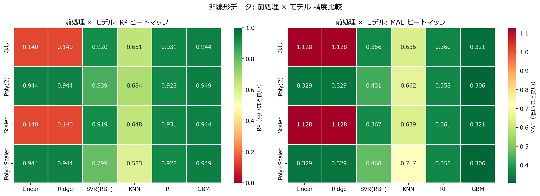
df_res = pd.DataFrame(results)

fig, axes = plt.subplots(1, 2, figsize=(14, 5))

pivot_r2 = df_res.pivot_table(index="前処理", columns="モデル", values="R²")
prep_order = ["なし", "Poly(2)", "Scaler", "Poly+Scaler"]
mdl_order = ["Linear", "Ridge", "SVR(RBF)", "KNN", "RF", "GBM"]
pivot_r2 = pivot_r2.reindex(index=[p for p in prep_order if p in pivot_r2.index],
                            columns=[m for m in mdl_order if m in pivot_r2.columns])

sns.heatmap(pivot_r2, annot=True, fmt=".3f", cmap="RdYlGn",
            linewidths=0.5, ax=axes[0], vmin=0, vmax=1,
            cbar_kws={"label": "R²（高いほど良い）"})
axes[0].set_title("前処理 × モデル: R² ヒートマップ")
axes[0].set_xlabel("")
axes[0].set_ylabel("")

pivot_mae = df_res.pivot_table(index="前処理", columns="モデル", values="MAE")
pivot_mae = pivot_mae.reindex(index=[p for p in prep_order if p in pivot_mae.index],
                              columns=[m for m in mdl_order if m in pivot_mae.columns])

sns.heatmap(pivot_mae, annot=True, fmt=".3f", cmap="RdYlGn_r",
            linewidths=0.5, ax=axes[1],
            cbar_kws={"label": "MAE（低いほど良い）"})
axes[1].set_title("前処理 × モデル: MAE ヒートマップ")
axes[1].set_xlabel("")
axes[1].set_ylabel("")

fig.suptitle("非線形データ: 前処理 × モデル 精度比較", fontsize=13)
fig.tight_layout()
plt.show()

 1
 2
 3
 4
 5
 6
 7
 8
 9
10
11
12
13
14
15
16
17
18
19
20
21
22
23
24
25
26
27
28
29

from sklearn.model_selection import train_test_split
from sklearn.base import clone

X_tr, X_te, y_tr, y_te = train_test_split(X, y, test_size=0.3, random_state=42)

configs = [
    ("Linear（生データ）", LinearRegression(), False, False),
    ("Ridge + Poly(2)", Ridge(alpha=1.0), True, False),
    ("GBM（生データ）", GradientBoostingRegressor(n_estimators=100, random_state=42), False, False),
]

fig, axes = plt.subplots(1, 3, figsize=(15, 4))
for i, (name, mdl, poly, scale) in enumerate(configs):
    pipe = make_pipeline(clone(mdl), poly=poly, scale=scale)
    pipe.fit(X_tr, y_tr)
    pred = pipe.predict(X_te)
    residuals = y_te - pred

    axes[i].scatter(pred, residuals, alpha=0.4, s=15, color="#2563eb")
    axes[i].axhline(0, color="#ef4444", linewidth=1, linestyle="--")
    r2 = 1 - np.sum(residuals**2) / np.sum((y_te - np.mean(y_te))**2)
    axes[i].set_title(f"{name}\nR²={r2:.3f}", fontsize=10)
    axes[i].set_xlabel("予測値")
    axes[i].set_ylabel("残差")
    axes[i].grid(alpha=0.2)

fig.suptitle("残差パターンの比較（テストデータ）", fontsize=13)
fig.tight_layout()
plt.show()