【ベンチマーク】外れ値を含む回帰

 1
 2
 3
 4
 5
 6
 7
 8
 9
10
11
12
13
14
15
16
17
18
19
20
21
22
23
24
25
26
27
28
29
30
31
32
33
34
35
36
37
38
39
40
41
42
43
44
45
46
47
48
49
50

import numpy as np
import pandas as pd
import matplotlib.pyplot as plt

rng = np.random.default_rng(42)
n = 300

X = rng.normal(0, 1, size=(n, 2))
y_clean = 2 * X[:, 0] + 3 * X[:, 1] + rng.normal(0, 1, size=n)

# 10%の外れ値を注入
y = y_clean.copy()
outlier_idx = rng.choice(n, size=int(n * 0.10), replace=False)
outlier_signs = rng.choice([-1, 1], size=len(outlier_idx))
y[outlier_idx] = outlier_signs * rng.uniform(20, 40, size=len(outlier_idx))

fig, axes = plt.subplots(1, 3, figsize=(15, 4))

# 散布図 x1 vs y
mask = np.zeros(n, dtype=bool)
mask[outlier_idx] = True
axes[0].scatter(X[~mask, 0], y[~mask], alpha=0.4, s=15, color="#2563eb", label="正常")
axes[0].scatter(X[mask, 0], y[mask], alpha=0.8, s=30, color="#ef4444", marker="x", label="外れ値")
axes[0].set_title("x₁ vs y")
axes[0].set_xlabel("x₁")
axes[0].set_ylabel("y")
axes[0].legend(fontsize=8)
axes[0].grid(alpha=0.2)

# 散布図 x2 vs y
axes[1].scatter(X[~mask, 1], y[~mask], alpha=0.4, s=15, color="#2563eb", label="正常")
axes[1].scatter(X[mask, 1], y[mask], alpha=0.8, s=30, color="#ef4444", marker="x", label="外れ値")
axes[1].set_title("x₂ vs y")
axes[1].set_xlabel("x₂")
axes[1].set_ylabel("y")
axes[1].legend(fontsize=8)
axes[1].grid(alpha=0.2)

# yの分布
axes[2].hist(y, bins=30, color="#2563eb", edgecolor="white", alpha=0.7)
axes[2].axvline(np.percentile(y, 5), color="#f97316", linestyle="--", label="5th / 95th %ile")
axes[2].axvline(np.percentile(y, 95), color="#f97316", linestyle="--")
axes[2].set_title(f"yの分布（外れ値 {len(outlier_idx)} 個）")
axes[2].set_xlabel("y")
axes[2].legend(fontsize=8)
axes[2].grid(alpha=0.2)

fig.suptitle("外れ値汚染データの構造", fontsize=13)
fig.tight_layout()
plt.show()

 1
 2
 3
 4
 5
 6
 7
 8
 9
10
11
12
13
14
15
16
17
18
19
20
21
22
23
24
25
26
27
28
29
30
31
32
33
34
35
36
37
38
39
40
41
42
43
44
45
46
47
48
49
50
51
52
53
54
55
56
57
58
59
60
61
62
63
64
65
66
67
68
69
70
71
72
73
74
75
76
77
78
79
80
81
82
83
84
85
86
87
88
89
90
91
92
93
94
95
96
97

from sklearn.model_selection import cross_val_score, KFold
from sklearn.linear_model import LinearRegression, Ridge, RANSACRegressor, HuberRegressor, TheilSenRegressor
from sklearn.base import clone
from scipy.stats import mstats
import seaborn as sns

cv = KFold(n_splits=5, shuffle=True, random_state=42)

models = {
    "OLS": LinearRegression(),
    "Ridge": Ridge(alpha=1.0),
    "RANSAC": RANSACRegressor(estimator=LinearRegression(), random_state=42),
    "Huber": HuberRegressor(epsilon=1.35),
    "TheilSen": TheilSenRegressor(random_state=42),
}

def iqr_filter(X, y):
    q1, q3 = np.percentile(y, 25), np.percentile(y, 75)
    iqr = q3 - q1
    mask = (y >= q1 - 1.5 * iqr) & (y <= q3 + 1.5 * iqr)
    return X[mask], y[mask]

def winsorize(y, pct=0.05):
    lower = np.percentile(y, pct * 100)
    upper = np.percentile(y, (1 - pct) * 100)
    return np.clip(y, lower, upper)

preprocs = {
    "なし": lambda X, y: (X, y),
    "IQR除去": iqr_filter,
    "Winsorize(5%)": lambda X, y: (X, winsorize(y)),
}

results = []
for prep_name, prep_fn in preprocs.items():
    for mdl_name, mdl in models.items():
        maes, coef_bias = [], []
        for train_idx, test_idx in cv.split(X):
            X_tr, X_te = X[train_idx], X[test_idx]
            y_tr, y_te = y[train_idx], y[test_idx]

            X_pp, y_pp = prep_fn(X_tr, y_tr)
            m = clone(mdl)
            try:
                m.fit(X_pp, y_pp)
                pred = m.predict(X_te)
                maes.append(np.mean(np.abs(y_te - pred)))

                # 係数バイアス
                if hasattr(m, "coef_"):
                    coefs = m.coef_.ravel()[:2] if len(m.coef_.ravel()) >= 2 else m.coef_.ravel()
                elif hasattr(m, "estimator_") and hasattr(m.estimator_, "coef_"):
                    coefs = m.estimator_.coef_.ravel()[:2]
                else:
                    coefs = [np.nan, np.nan]
                true_coefs = np.array([2.0, 3.0])
                bias = np.mean(np.abs(coefs[:2] - true_coefs[:2]))
                coef_bias.append(bias)
            except Exception:
                maes.append(np.nan)
                coef_bias.append(np.nan)

        results.append({
            "前処理": prep_name, "モデル": mdl_name,
            "MAE": np.nanmean(maes),
            "係数バイアス": np.nanmean(coef_bias),
        })

df_res = pd.DataFrame(results)

fig, axes = plt.subplots(1, 2, figsize=(14, 4.5))

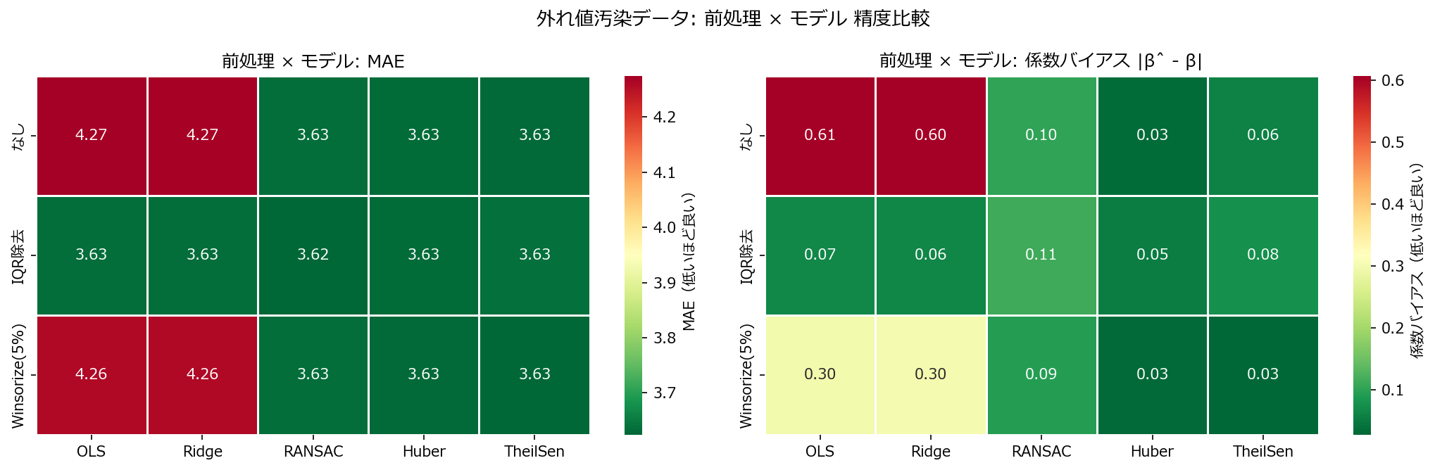
pivot_mae = df_res.pivot_table(index="前処理", columns="モデル", values="MAE")
prep_order = ["なし", "IQR除去", "Winsorize(5%)"]
mdl_order = ["OLS", "Ridge", "RANSAC", "Huber", "TheilSen"]
pivot_mae = pivot_mae.reindex(index=[p for p in prep_order if p in pivot_mae.index],
                              columns=[m for m in mdl_order if m in pivot_mae.columns])

sns.heatmap(pivot_mae, annot=True, fmt=".2f", cmap="RdYlGn_r",
            linewidths=0.5, ax=axes[0], cbar_kws={"label": "MAE（低いほど良い）"})
axes[0].set_title("前処理 × モデル: MAE")
axes[0].set_xlabel("")
axes[0].set_ylabel("")

pivot_bias = df_res.pivot_table(index="前処理", columns="モデル", values="係数バイアス")
pivot_bias = pivot_bias.reindex(index=[p for p in prep_order if p in pivot_bias.index],
                                columns=[m for m in mdl_order if m in pivot_bias.columns])

sns.heatmap(pivot_bias, annot=True, fmt=".2f", cmap="RdYlGn_r",
            linewidths=0.5, ax=axes[1], cbar_kws={"label": "係数バイアス（低いほど良い）"})
axes[1].set_title("前処理 × モデル: 係数バイアス |β̂ - β|")
axes[1].set_xlabel("")
axes[1].set_ylabel("")

fig.suptitle("外れ値汚染データ: 前処理 × モデル 精度比較", fontsize=13)
fig.tight_layout()
plt.show()

 1
 2
 3
 4
 5
 6
 7
 8
 9
10
11
12
13
14
15
16
17
18
19
20
21
22
23
24
25
26
27
28
29
30
31
32
33
34
35

from sklearn.model_selection import train_test_split
from sklearn.base import clone

X_tr, X_te, y_tr, y_te = train_test_split(X, y, test_size=0.3, random_state=42)
_, _, y_clean_tr, y_clean_te = train_test_split(X, y_clean, test_size=0.3, random_state=42)

configs = [
    ("OLS（生データ）", LinearRegression(), "なし"),
    ("RANSAC（生データ）", RANSACRegressor(estimator=LinearRegression(), random_state=42), "なし"),
    ("OLS + IQR除去", LinearRegression(), "IQR"),
]

fig, axes = plt.subplots(1, 3, figsize=(15, 4))
for i, (name, mdl, prep) in enumerate(configs):
    m = clone(mdl)
    if prep == "IQR":
        X_fit, y_fit = iqr_filter(X_tr, y_tr)
    else:
        X_fit, y_fit = X_tr, y_tr

    m.fit(X_fit, y_fit)
    pred = m.predict(X_te)
    residuals = y_clean_te - pred  # 真の値からの残差

    axes[i].scatter(pred, residuals, alpha=0.4, s=15, color="#2563eb")
    axes[i].axhline(0, color="#ef4444", linewidth=1, linestyle="--")
    mae = np.mean(np.abs(residuals))
    axes[i].set_title(f"{name}\nMAE(vs真値)={mae:.2f}", fontsize=10)
    axes[i].set_xlabel("予測値")
    axes[i].set_ylabel("残差（真の値 - 予測）")
    axes[i].grid(alpha=0.2)

fig.suptitle("残差パターンの比較（テストデータ, 真の値に対する残差）", fontsize=13)
fig.tight_layout()
plt.show()