線形回帰と最小二乗法 | 基礎理論とPython実装

まとめ

線形回帰は入力と出力の線形関係をモデル化する最も基本的な回帰モデルであり、予測と解釈の両方に使える。
最小二乗法は残差二乗和を最小化することで係数を推定し、解析的な解が得られるため仕組みが理解しやすい。
傾き係数は「入力が 1 増えたとき出力がどれだけ変化するか」、切片は入力が 0 のときの期待値として解釈できる。
ノイズや外れ値が大きい場合には標準化やロバスト手法も検討し、前処理と評価指標を組み合わせて活用する。

直感 #

観測されたデータ $(x_i, y_i)$ が散布図上でほぼ直線状に並ぶとき、未知の入力に対しても直線を延長すればよいのではないか、という素朴な発想から生まれたのが線形回帰です。最小二乗法はプロットした点の近くに一本の直線を引き、その直線からのズレが全体として最も小さくなるように傾きと切片を選びます。

具体的な数式 #

一次の線形モデルは

$$ y = w x + b $$

で表されます。観測値と予測値の差（残差）$\epsilon_i = y_i - (w x_i + b)$ の二乗和を目的関数

$$ L(w, b) = \sum_{i=1}^{n} \big(y_i - (w x_i + b)\big)^2 $$

として最小化すると、解析的に次の解が得られます。

$$ w = \frac{\sum_{i=1}^{n} (x_i - \bar{x})(y_i - \bar{y})}{\sum_{i=1}^{n} (x_i - \bar{x})^2}, \qquad b = \bar{y} - w \bar{x} $$

ここで $\bar{x}, \bar{y}$ はそれぞれの平均です。複数の入力を使う重回帰でも、ベクトルと行列を用いて同様に最小二乗解を導くことができます。

Pythonを用いた実験や説明 #

次のコードは scikit-learn を使って単回帰モデルを学習し、推定された直線と観測値を描画します。コード本体は既存のものをそのまま利用しています。

from __future__ import annotations

import japanize_matplotlib
import matplotlib.pyplot as plt
import numpy as np
from sklearn.linear_model import LinearRegression
from sklearn.pipeline import make_pipeline
from sklearn.preprocessing import StandardScaler


def plot_simple_linear_regression(n_samples: int = 100) -> None:
    """Plot a fitted linear regression model for synthetic data.

    Args:
        n_samples: Number of synthetic samples to generate.
    """
    japanize_matplotlib.japanize()
    rng = np.random.default_rng(seed=0)

    X: np.ndarray = np.linspace(-5.0, 5.0, n_samples, dtype=float)[:, np.newaxis]
    noise: np.ndarray = rng.normal(scale=2.0, size=n_samples)
    y: np.ndarray = 2.0 * X.ravel() + 1.0 + noise

    model = make_pipeline(StandardScaler(with_mean=False), LinearRegression())
    model.fit(X, y)
    y_pred: np.ndarray = model.predict(X)

    fig, ax = plt.subplots(figsize=(10, 5))
    ax.scatter(X, y, marker="x", label="Observed data", c="orange")
    ax.plot(X, y_pred, label="Regression fit")
    ax.set_xlabel("$x$")
    ax.set_ylabel("$y$")
    ax.legend()
    fig.tight_layout()
    plt.show()

plot_simple_linear_regression()

コード本体は既存のものをそのまま利用していますの図

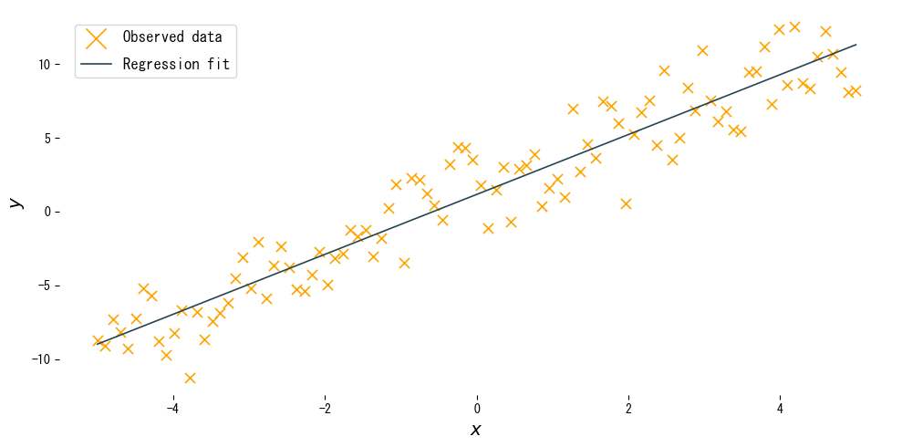
実行結果の読み方 #

傾き $w$: 入力が 1 増えたときに出力がどれだけ増減するかを表し、真の傾きに近い値が推定されます。
切片 $b$: 入力が 0 のときの平均的な出力であり、直線の位置を上下に調整します。
StandardScaler で特徴量を標準化すると、スケールの異なる入力でも安定して学習できます。

参考文献 #

Draper, N. R., & Smith, H. (1998). Applied Regression Analysis (3rd ed.). John Wiley & Sons.
Hastie, T., Tibshirani, R., & Friedman, J. (2009). The Elements of Statistical Learning. Springer.