主成分回帰 (PCR) | 多重共線性を緩和する次元圧縮回帰

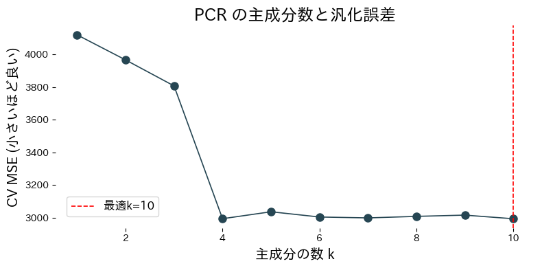
from __future__ import annotations

import japanize_matplotlib
import matplotlib.pyplot as plt
import numpy as np
from sklearn.datasets import load_diabetes
from sklearn.decomposition import PCA
from sklearn.linear_model import LinearRegression
from sklearn.model_selection import cross_val_score
from sklearn.pipeline import Pipeline
from sklearn.preprocessing import StandardScaler


def evaluate_pcr_components(
    cv_folds: int = 5,
    xlabel: str = "Number of components k",
    ylabel: str = "CV MSE (lower is better)",
    title: str | None = None,
    label_best: str = "best={k}",
) -> dict[str, float]:
    """Cross-validate PCR with varying component counts and plot the curve.

    Args:
        cv_folds: Number of folds for cross-validation.
        xlabel: Label for the component-count axis.
        ylabel: Label for the error axis.
        title: Optional title for the plot.
        label_best: Format string for highlighting the best component count.

    Returns:
        Dictionary containing the best component count and its CV score.
    """
    japanize_matplotlib.japanize()
    X, y = load_diabetes(return_X_y=True)

    def build_pcr(n_components: int) -> Pipeline:
        return Pipeline([
            ("scale", StandardScaler()),
            ("pca", PCA(n_components=n_components, random_state=0)),
            ("reg", LinearRegression()),
        ])

    components = np.arange(1, X.shape[1] + 1)
    cv_scores = []
    for k in components:
        model = build_pcr(int(k))
        score = cross_val_score(
            model,
            X,
            y,
            cv=cv_folds,
            scoring="neg_mean_squared_error",
        )
        cv_scores.append(score.mean())

    cv_scores_arr = np.array(cv_scores)
    best_idx = int(np.argmax(cv_scores_arr))
    best_k = int(components[best_idx])
    best_mse = float(-cv_scores_arr[best_idx])

    best_model = build_pcr(best_k).fit(X, y)
    explained = best_model["pca"].explained_variance_ratio_

    fig, ax = plt.subplots(figsize=(8, 4))
    ax.plot(components, -cv_scores_arr, marker="o")
    ax.axvline(best_k, color="red", linestyle="--", label=label_best.format(k=best_k))
    ax.set_xlabel(xlabel)
    ax.set_ylabel(ylabel)
    if title:
        ax.set_title(title)
    ax.legend()
    fig.tight_layout()
    plt.show()

    return {
        "best_k": best_k,
        "best_mse": best_mse,
        "explained_variance_ratio": explained,
    }



metrics = evaluate_pcr_components(
    xlabel="主成分の数 k",
    ylabel="CV MSE (小さいほど良い)",
    title="PCR の主成分数と汎化誤差",
    label_best="最適k={k}",
)
print(f"最適な主成分数: {metrics['best_k']}")
print(f"最適CV MSE: {metrics['best_mse']:.3f}")
print("寄与率:", metrics['explained_variance_ratio'])