加重最小二乗法 (WLS)

最終更新 2020-06-17 読了時間 3 分

まとめ

加重最小二乗法 (WLS) は観測ごとの信頼度に応じて重みを割り当て、異質なノイズを持つデータでも妥当な回帰直線を推定する。
重みを二乗誤差に掛けることで、分散の小さい観測ほど強く反映され、ノイズの大きい点に引きずられにくくなる。
標準の LinearRegression に sample_weight を指定すれば WLS を実行できる。
重みは既知の分散、残差の推定、ドメイン知識など複数の観点を組み合わせて設計する。

直感 #

通常の最小二乗法はすべての観測が同じ信頼度を持つと仮定します。しかし実務では、センサー性能や測定回数によって精度が大きく異なることがよくあります。WLS は「信頼できる点の意見をより尊重する」ように重みを付け直し、線形回帰の枠組みで異質なデータを扱います。

具体的な数式 #

観測ごとに重み $w_i > 0$ を与えて目的関数

$$ L(\boldsymbol\beta, b) = \sum_{i=1}^{n} w_i \left(y_i - (\boldsymbol\beta^\top \mathbf{x}_i + b)\right)^2 $$

を最小化します。理想的には $w_i \propto 1/\sigma_i^2$（分散の逆数）と設定し、信頼度の高いデータ点ほど重みを大きくします。

Pythonを用いた実験や説明 #

ノイズレベルが区間で異なるデータに WLS を適用する例です。

 1
 2
 3
 4
 5
 6
 7
 8
 9
10
11
12
13
14
15
16
17
18
19
20
21
22
23
24
25
26
27
28
29
30
31
32
33
34
35
36
37
38
39
40
41
42
43
44
45
46
47
48
49
50
51
52
53
54
55
56
57
58
59
60
61
62
63
64
65
66
67
68
69
70
71
72
73
74
75
76
77
78
79
80
81
82
83
84
85
86
87
88
89
90
91
92
93
94
95
96
from __future__ import annotations

import matplotlib.pyplot as plt
import numpy as np
from sklearn.linear_model import LinearRegression

def run_weighted_vs_ols(
    n_samples: int = 200,
    threshold: float = 5.0,
    low_noise: float = 0.5,
    high_noise: float = 2.5,
    xlabel: str = "input $",
    ylabel: str = "output $",
    label_scatter: str = "observations (color=noise)",
    label_truth: str = "true line",
    label_ols: str = "OLS",
    label_wls: str = "WLS",
    title: str | None = None,
) -> dict[str, float]:
    """Compare OLS and weighted least squares on heteroscedastic data.

    Args:
        n_samples: Number of evenly spaced samples to generate.
        threshold: Breakpoint separating low- and high-noise regions.
        low_noise: Noise scale for the lower region.
        high_noise: Noise scale for the higher region.
        xlabel: Label for the x-axis.
        ylabel: Label for the y-axis.
        label_scatter: Legend label for the colored scatter plot.
        label_truth: Legend label for the ground-truth line.
        label_ols: Legend label for the OLS fit.
        label_wls: Legend label for the WLS fit.
        title: Optional title for the plot.

    Returns:
        Dictionary with slopes and intercepts of both fits.
    """
    rng = np.random.default_rng(7)

    X_vals: np.ndarray = np.linspace(0.0, 10.0, n_samples, dtype=float)
    true_y: np.ndarray = 1.2 * X_vals + 3.0

    noise_scale = np.where(X_vals < threshold, low_noise, high_noise)
    y_noisy = true_y + rng.normal(scale=noise_scale)

    weights = 1.0 / (noise_scale**2)
    X = X_vals[:, np.newaxis]

    ols = LinearRegression()
    ols.fit(X, y_noisy)

    wls = LinearRegression()
    wls.fit(X, y_noisy, sample_weight=weights)

    grid = np.linspace(0.0, 10.0, 200, dtype=float)[:, np.newaxis]
    ols_pred = ols.predict(grid)
    wls_pred = wls.predict(grid)

    fig, ax = plt.subplots(figsize=(10, 5))
    scatter = ax.scatter(
        X,
        y_noisy,
        c=noise_scale,
        cmap="coolwarm",
        s=25,
        label=label_scatter,
    )
    ax.plot(grid, 1.2 * grid.ravel() + 3.0, color="#2ca02c", label=label_truth)
    ax.plot(grid, ols_pred, color="#1f77b4", linestyle="--", linewidth=2, label=label_ols)
    ax.plot(grid, wls_pred, color="#d62728", linewidth=2, label=label_wls)
    ax.set_xlabel(xlabel)
    ax.set_ylabel(ylabel)
    if title:
        ax.set_title(title)
    ax.legend()
    fig.tight_layout()
    plt.show()

    return {
        "ols_slope": float(ols.coef_[0]),
        "ols_intercept": float(ols.intercept_),
        "wls_slope": float(wls.coef_[0]),
        "wls_intercept": float(wls.intercept_),
    }

metrics = run_weighted_vs_ols(
    xlabel="入力 $",
    ylabel="出力 $",
    label_scatter="観測値 (色=ノイズ)",
    label_truth="真の直線",
    label_ols="OLS",
    label_wls="WLS",
    title="重み付き最小二乗法とOLSの比較",
)
print(f"OLS の傾き: {metrics['ols_slope']:.3f}, 切片: {metrics['ols_intercept']:.3f}")
print(f"WLS の傾き: {metrics['wls_slope']:.3f}, 切片: {metrics['wls_intercept']:.3f}")

ノイズレベルが区間で異なるデータに WLS を適用する例ですの図

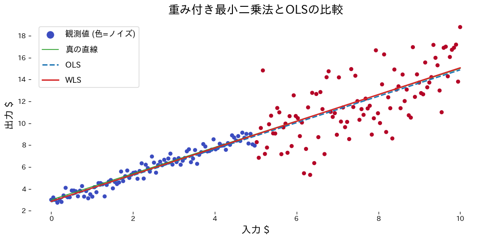
実行結果の読み方 #

weights を与えることでノイズの小さい区間がより重視され、真の直線に近い推定になる。
OLS の直線はノイズの大きい区間に引っ張られ、傾きが過小評価されやすい。
重みを適切に設定することが性能改善の鍵となる。

よくある質問 #

OLSとWLSはどう使い分ける？ #

OLS（通常最小二乗法）は全観測が等分散であることを前提とします。残差プロットで分散が入力値に依存して変化する（不均一分散、ヘテロスケダスティシティ）ことが確認された場合にWLSを使います。Breusch-PaganテストやWhiteテストで不均一分散を統計的に検定してから判断するのが標準的です。

重みの決め方は？ #

主な設定方法：

分散の逆数：各観測の誤差分散が既知または推定できる場合は $w_i = 1/\hat{\sigma}_i^2$
測定回数の平方根：複数回測定の平均値を使う場合は測定回数 $n_i$ を重みに
残差の逆数：2段階推定（まずOLS残差を計算し、残差の絶対値の逆数を重みに）
ドメイン知識：センサー精度や信頼度スコアなど外部情報から設計

WLSとGLSの違いは？ #

WLS（加重最小二乗法）は誤差の分散のみが観測ごとに異なる場合（対角共分散行列）を扱います。GLS（一般化最小二乗法）は誤差間に相関がある場合も含む一般的な枠組みで、WLSはGLSの特殊ケースです。時系列の自己相関がある場合はFeasible GLS（FGLS）が必要です。

sklearnでWLSを実行するには？ #

LinearRegression.fit(X, y, sample_weight=weights)のsample_weight引数に重みベクトルを渡すだけです。重みは正の値で、分散の逆数（1 / sigma**2）として設定するのが理想的です。

参考文献 #

Carroll, R. J., & Ruppert, D. (1988). Transformation and Weighting in Regression. Chapman & Hall.
Seber, G. A. F., & Lee, A. J. (2012). Linear Regression Analysis (2nd ed.). Wiley.