まとめ 回帰木は特徴量空間を条件分岐で細かく分割し、各葉ノードで目標値の代表値(平均や中央値など)を返す 分割は平均二乗誤差などの指標がどれだけ減るかで評価し、減少量が最大の特徴量としきい値を選ぶ 予測関数は段差状になるため、深さや葉あたりのサンプル数を調整して当てはまりと汎化性能を両立させる 木構造を可視化すると、どの特徴量がどの範囲で値に影響しているかを直感的に把握できる 直感
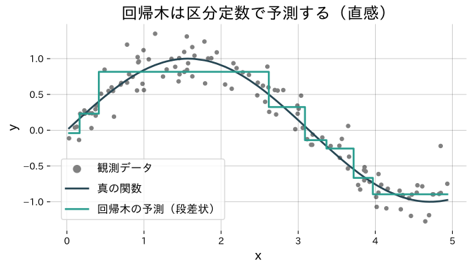
# 決定木分類と同様に「もし◯◯なら左へ」と特徴量を基準に分岐しますが、葉ノードでは連続値を返します。葉に含まれるサンプルの平均(criterion="squared_error" の場合)などが予測値になるため、出力は段差状の区分的な関数になります。木を深くすると細かな変化も表現できますが、過学習しやすいので枝刈りや深さ制限で滑らかさを調整します。
flowchart TD
A["根ノード"] --> B["特徴量と\n閾値を選択"]
B --> C["MSE減少量\nを最大化"]
C --> D{"深さ制限\nに到達?"}
D -->|No| B
D -->|Yes| E["葉ノード\n(平均値を返す)"]
style A fill:#2563eb,color:#fff
style C fill:#1e40af,color:#fff
style E fill:#10b981,color:#fff
具体的な数式
# ノード \(t\) における平均二乗誤差 \(\mathrm{MSE}(t)\) は
$$
\mathrm{MSE}(t) = \frac{1}{n_t} \sum_{i \in t} \bigl(y_i - \bar{y}_t\bigr)^2
$$で定義されます。親ノード \(t\) を特徴量 \(x_j\) としきい値 \(s\) で左右に分割したとき、不純度減少量
$$
\Delta = \mathrm{MSE}(t)
\frac{n_L}{n_t} \mathrm{MSE}(t_L) \frac{n_R}{n_t} \mathrm{MSE}(t_R)
$$ が最大になる組み合わせを選ぶことで、段差状の近似関数が得られます。葉ノードでは \(\bar{y}_t\)(または中央値など)を予測値とします。
Pythonを用いた実験や説明
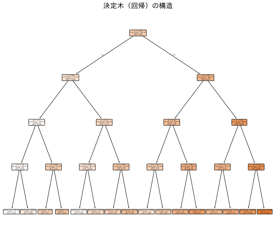
# 最初のコードはノイズ付きの 1 次元データに深さ 3 の回帰木を当てはめ、段差状の予測がどのように真の関数を近似するかを確認します。続くコードでは 2 特徴量の回帰データで予測面を等高線として可視化し、木を深くしたときの評価指標(\(R^2\)、RMSE、MAE)を出力します。
 1
 2
 3
 4
 5
 6
 7
 8
 9
10
11
12
13
14
15
16
17
18
19
20
21
22
23
24
25
import numpy as np
import matplotlib.pyplot as plt
from sklearn.tree import DecisionTreeRegressor , plot_tree
from sklearn.datasets import make_regression
from sklearn.metrics import r2_score , mean_squared_error , mean_absolute_error
# 1 次元ノイズ付きデータ
rng = np . random . default_rng ( 42 )
X1 = np . sort ( 5 * rng . random (( 120 , 1 )), axis = 0 )
y1_true = np . sin ( X1 ) . ravel ()
y1 = y1_true + rng . normal ( scale = 0.2 , size = X1 . shape [ 0 ])
reg1 = DecisionTreeRegressor ( max_depth = 3 , random_state = 0 ) . fit ( X1 , y1 )
y1_pred = reg1 . predict ( X1 )
plt . figure ( figsize = ( 8 , 4 ))
plt . scatter ( X1 , y1 , s = 15 , c = "gray" , label = "観測値" )
plt . plot ( X1 , y1_true , lw = 2 , label = "真の関数" )
plt . step ( X1 . ravel (), y1_pred , where = "mid" , lw = 2 , label = "回帰木の予測" )
plt . xlabel ( "x" )
plt . ylabel ( "y" )
plt . title ( "回帰木は区分的な関数として振る舞う" )
plt . legend ()
plt . grid ( alpha = 0.3 )
plt . show ()
 1
 2
 3
 4
 5
 6
 7
 8
 9
10
11
12
13
14
15
16
17
18
19
20
21
22
23
24
25
26
27
# 2 特徴量の回帰データ
X , y = make_regression ( n_samples = 400 , n_features = 2 , noise = 15.0 , random_state = 777 )
reg = DecisionTreeRegressor ( max_depth = 4 , random_state = 0 ) . fit ( X , y )
# 評価指標
r2 = r2_score ( y , reg . predict ( X ))
rmse = mean_squared_error ( y , reg . predict ( X ), squared = False )
mae = mean_absolute_error ( y , reg . predict ( X ))
print ( f "R2= { r2 : .3f } RMSE= { rmse : .2f } MAE= { mae : .2f } " )
# 等高線で予測面を可視化
x_min , x_max = X [:, 0 ] . min () - 1 , X [:, 0 ] . max () + 1
y_min , y_max = X [:, 1 ] . min () - 1 , X [:, 1 ] . max () + 1
xx , yy = np . meshgrid (
np . linspace ( x_min , x_max , 150 ),
np . linspace ( y_min , y_max , 150 ),
)
zz = reg . predict ( np . c_ [ xx . ravel (), yy . ravel ()]) . reshape ( xx . shape )
plt . figure ( figsize = ( 7 , 6 ))
cs = plt . contourf ( xx , yy , zz , levels = 15 , cmap = "viridis" , alpha = 0.8 )
plt . colorbar ( cs , label = "予測値" )
plt . scatter ( X [:, 0 ], X [:, 1 ], c = y , cmap = "viridis" , s = 20 , edgecolor = "k" , alpha = 0.7 )
plt . xlabel ( "x1" )
plt . ylabel ( "x2" )
plt . title ( "回帰木の予測面(等高線表示)" )
plt . show ()
1
2
3
4
5
6
7
8
plt . figure ( figsize = ( 12 , 10 ))
plot_tree (
reg , filled = True ,
feature_names = [ "x1" , "x2" ],
rounded = True ,
)
plt . title ( "決定木回帰の構造" )
plt . show ()
回帰木は深くしすぎると訓練データのノイズまで拾い、過学習します。max_depthやmin_samples_leafを制限し、交差検証でチューニングしてください。また出力が段差状になるため、滑らかな関数の近似には多数の木を組み合わせるアンサンブル手法(勾配ブースティングやランダムフォレスト)が有効です。
plot_treeで木構造を可視化すると、どの特徴量がどの範囲で予測に寄与しているかを直感的に把握できます。max_depth=3〜5程度に抑えると解釈性と精度のバランスが取りやすくなります。
最大深さと回帰曲線
# 決定木の深さを増やすとステップ関数がどう細かくなるか確認できます。
まとめ
# 回帰木は特徴量空間を条件分岐で分割し、各葉ノードで目標値の平均を返す区分的な関数です。 分割はMSE減少量が最大になる特徴量と閾値の組み合わせを貪欲に選びます。 深い木は過学習しやすいため、max_depthやmin_samples_leafによる制約が重要です。 木構造の可視化により、予測の根拠を直感的に説明できる解釈性の高いモデルです。 参考文献
# Breiman, L., Friedman, J. H., Olshen, R. A., & Stone, C. J. (1984). Classification and Regression Trees . Wadsworth. scikit-learn developers. (2024). Decision Trees . https://scikit-learn.org/stable/modules/tree.html