決定木のパラメータ

直感 #

決定木は「\(x_1 \le 0.3\) なら左へ、そうでなければ右へ」と条件を繰り返し、葉ノードで値を返します。制限を設けなければ 500 点の訓練データを 500 枚の葉で覆ってほぼ完璧に再現できますが、そのぶんノイズ 1 点のために作られた葉が増え、テストデータでは外れます。max_depth=3 は「質問は 3 回まで」、min_samples_leaf=5 は「5 点未満の部屋は作らない」という意味で、どちらも葉の数を減らして予測面を粗くする方向に働きます。ccp_alpha だけは発想が逆で、いったん育て切った木から「葉 1 枚を減らして増える誤差が \(\alpha\) 未満なら刈る」を繰り返します。

何が起きているか（ステップで見る） #

コードを読む前に、この手法が図の上で何をしているかを追ってみましょう。「再生」を押すか、スライダーを動かすと 1 手順ずつ進みます。

見るポイント：切る線は必ず軸に平行で、max_depth は「何本目の線で止めるか」に当たります。深さを増やしても誤分類の数が減らなくなった手順から先が過学習の領域で、min_samples_leaf を 5 にすれば点が 5 個未満の小さな部屋は作られなくなります。

式で書くと何を基準に止めているか #

どのパラメータも、分割を続けるか止めるかの判断に介入します。親ノード \(P\) を左右の子ノード \(L, R\) に分割したときの不純度減少量は

で表されます。回帰木の場合、\(I(t)\) を平均二乗誤差や平均絶対誤差として定義し、\(\Delta I\) が最大となる特徴量としきい値を選びます。max_depth は分割の回数、min_samples_leaf は \(|L|\) と \(|R|\) の下限、min_impurity_decrease は \(\Delta I\) の下限として、この分割を打ち切ります。

剪定では木 \(T\) のコスト複雑度

を最小化する部分木を探します。ここで \(R(T)\) は訓練誤差、\(|T|\) は葉ノード数、\(\alpha \ge 0\) は複雑さへのペナルティを表します。\(\alpha = 0\) なら育て切った木がそのまま残り、\(\alpha\) を大きくするほど「葉 1 枚あたりの誤差削減が \(\alpha\) に満たない枝」から順に刈られます。DecisionTreeRegressor(ccp_alpha=0.01) はこの \(\alpha\) を直接指定する引数です。

Pythonを用いた実験や説明 #

次のコードは 2 特徴量・500 点の回帰データを 7:3 に分け、max_depth、min_samples_leaf、ccp_alpha の 4 通りの設定で訓練 \(R^2\) とテスト \(R^2\) を並べて表示します。訓練とテストの差が大きい設定ほど過学習しています。

 1
 2
 3
 4
 5
 6
 7
 8
 9
10
11
12
13
14
15
16
17
18
19
20
21
22
23
24
25

import numpy as np
import matplotlib.pyplot as plt
from sklearn.model_selection import train_test_split
from sklearn.tree import DecisionTreeRegressor
from sklearn.datasets import make_regression
from sklearn.metrics import r2_score

X, y = make_regression(
    n_samples=500,
    n_features=2,
    noise=0.2,
    random_state=42,
)
Xtr, Xte, ytr, yte = train_test_split(X, y, test_size=0.3, random_state=0)

def evaluate(params):
    model = DecisionTreeRegressor(random_state=0, **params).fit(Xtr, ytr)
    r2_train = r2_score(ytr, model.predict(Xtr))
    r2_test = r2_score(yte, model.predict(Xte))
    print(f"{params}: train R2={r2_train:.3f}, test R2={r2_test:.3f}")

evaluate({"max_depth": 3})
evaluate({"max_depth": 10})
evaluate({"max_depth": 5, "min_samples_leaf": 5})
evaluate({"max_depth": 5, "ccp_alpha": 0.01})

実行結果の読み方 #

4 行の出力は、どの行も train R2 が test R2 以上になります。見るべきはその差で、max_depth=10 の行がいちばん開き、max_depth=3 や min_samples_leaf=5 の行は差が小さくなります。テスト \(R^2\) がいちばん高い設定が「このデータに合った複雑さ」で、実務では GridSearchCV で max_depth と min_samples_leaf の組み合わせを交差検証で選びます。

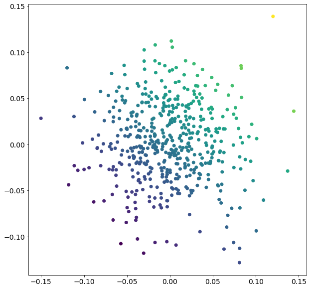
可視化ギャラリー #

以下の画像は過去に作成したノートブックを再利用したもので、max_depth、min_samples_leaf、ccp_alpha などの設定を変えたときの決定境界や予測面の違いをまとめています。深さを増やすほど長方形の領域が細かくなり、min_samples_leaf を大きくするほど小さな領域が消えることを見比べてください。

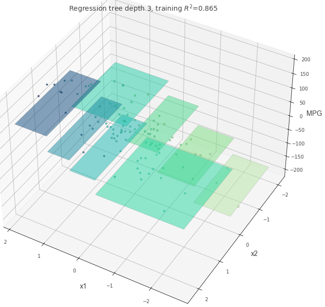
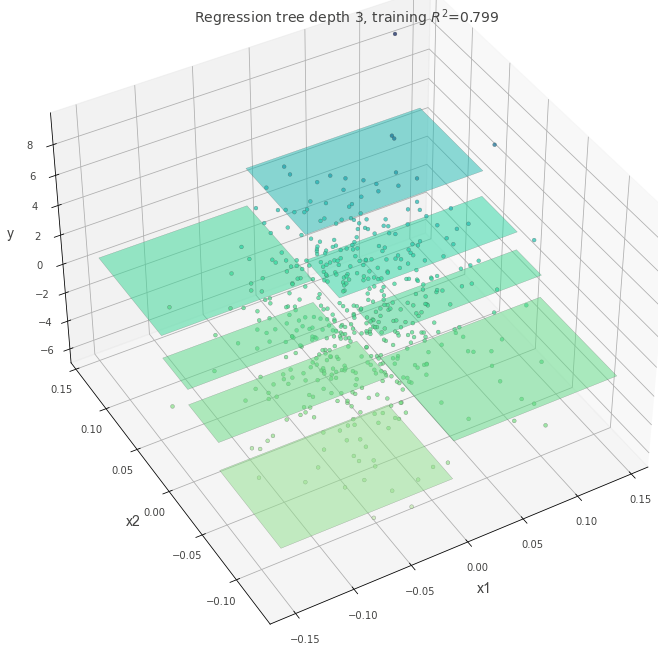
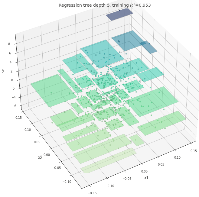
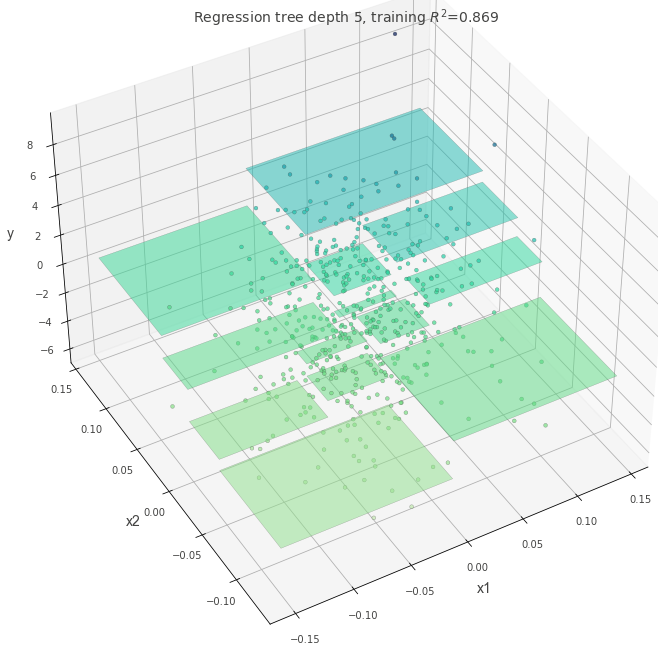
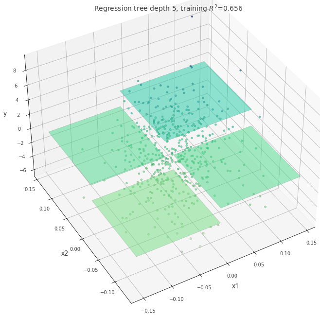
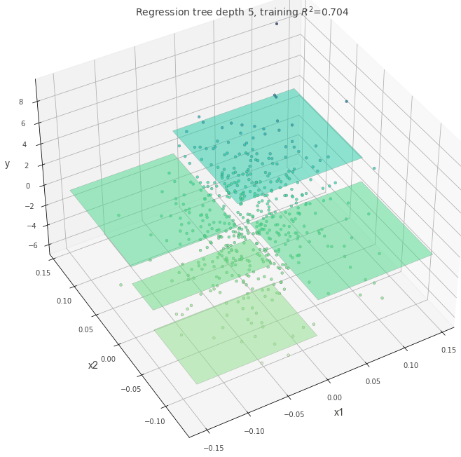
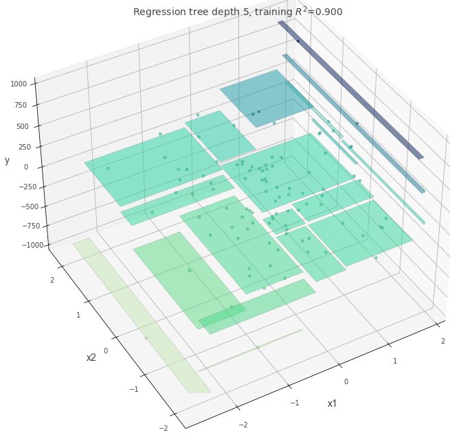
深さとモデルの複雑さ #

スライダーで max_depth を増やすと、訓練精度は単調に上がる一方でテスト精度は途中から頭打ちになり、2 つの線が乖離していく様子を確認できます。

まとめ #

決定木のパラメータは、不純度減少量 \(\Delta I\) による分割を「どこで止めるか」の設定です。max_depth は分割の回数、min_samples_leaf は葉のサンプル数の下限で、どちらも事前に成長を抑えます。ccp_alpha は育て切った木から \(R(T) + \alpha |T|\) が小さくなるよう事後に刈る剪定で、\(\alpha\) を大きくするほど葉が減ります。どの設定が良いかは訓練 \(R^2\) ではなくテスト \(R^2\) で判断し、1 本の木で安定しないときは ランダムフォレスト へ進みます。

参考文献 #