Μοντέλα Γκαουσιανής Μίξης (GMM)

Ενημέρωση 2020-03-25 Ανάγνωση 3 λεπτά

Σύνοψη

Ένα Μοντέλο Γκαουσιανής Μίξης αναπαριστά τα δεδομένα ως σταθμισμένο άθροισμα πολυμεταβλητών κανονικών συνιστωσών.
Παράγει έναν πίνακα ευθυνών που ποσοτικοποιεί πόσο ισχυρά κάθε συνιστώσα εξηγεί κάθε δείγμα.
Οι παράμετροι εκτιμώνται με τον αλγόριθμο EM· οι δομές συνδιακύμανσης μπορεί να είναι full, tied, diag ή spherical.
Η επιλογή μοντέλου συνήθως συνδυάζει κριτήρια πληροφορίας (BIC/AIC) με πολλαπλές τυχαίες αρχικοποιήσεις για σταθερότητα.

Εισαγωγή #

Αυτή η μέθοδος πρέπει να ερμηνεύεται μέσα από τις υποθέσεις της, τις συνθήκες δεδομένων και τον τρόπο με τον οποίο οι επιλογές παραμέτρων επηρεάζουν τη γενίκευση.

Αναλυτική Επεξήγηση #

Μαθηματική Διατύπωση #

Η πυκνότητα του $\mathbf{x}$ είναι

$$ p(\mathbf{x}) = \sum_{k=1}^{K} \pi_k \, \mathcal{N}(\mathbf{x} \mid \boldsymbol{\mu}_k, \boldsymbol{\Sigma}_k), $$

με βάρη μίξης $\pi_k$ (μη αρνητικά και με άθροισμα 1). Ο EM εναλλάσσει:

Βήμα E: υπολογισμός ευθυνών $\gamma_{ik}$. $$ \gamma_{ik} = \frac{\pi_k \, \mathcal{N}(\mathbf{x}_i \mid \boldsymbol{\mu}_k, \boldsymbol{\Sigma}_k)} {\sum_{j=1}^K \pi_j \, \mathcal{N}(\mathbf{x}_i \mid \boldsymbol{\mu}_j, \boldsymbol{\Sigma}_j)}. $$
Βήμα M: επανεκτίμηση $\pi_k, \boldsymbol{\mu}_k, \boldsymbol{\Sigma}k$ χρησιμοποιώντας $\gamma{ik}$ ως βάρη.

Η λογαριθμική πιθανοφάνεια αυξάνεται μονοτονικά και συγκλίνει σε τοπικό βέλτιστο.

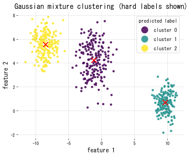
Πειράματα σε Python #

Προσαρμόζουμε ένα GMM σε συνθετικά δισδιάστατα σύννεφα σημείων, σχεδιάζουμε τις σκληρές αναθέσεις και αναφέρουμε τα βάρη μίξης και το σχήμα του πίνακα ευθυνών.

from __future__ import annotations

import matplotlib.pyplot as plt
import numpy as np
from numpy.typing import NDArray
from sklearn.datasets import make_blobs
from sklearn.mixture import GaussianMixture

def run_gmm_demo(
    n_samples: int = 600,
    n_components: int = 3,
    cluster_std: list[float] | tuple[float, ...] = (1.0, 1.4, 0.8),
    covariance_type: str = "full",
    random_state: int = 7,
    n_init: int = 8,
) -> dict[str, object]:
    """Fit a Gaussian mixture model and visualise hard labels with component centres."""
    features, _ = make_blobs(
        n_samples=n_samples,
        centers=n_components,
        cluster_std=cluster_std,
        random_state=random_state,
    )

    gmm = GaussianMixture(
        n_components=n_components,
        covariance_type=covariance_type,
        random_state=random_state,
        n_init=n_init,
    )
    gmm.fit(features)

    hard_labels = gmm.predict(features)
    responsibilities = gmm.predict_proba(features)
    log_likelihood = float(gmm.score(features))
    weights = gmm.weights_

    fig, ax = plt.subplots(figsize=(6.2, 5.2))
    scatter = ax.scatter(
        features[:, 0],
        features[:, 1],
        c=hard_labels,
        cmap="viridis",
        s=30,
        edgecolor="white",
        linewidth=0.2,
        alpha=0.85,
    )
    ax.scatter(
        gmm.means_[:, 0],
        gmm.means_[:, 1],
        marker="x",
        c="red",
        s=140,
        linewidth=2.0,
        label="Component centre",
    )
    ax.set_title("Gaussian mixture clustering (hard labels shown)")
    ax.set_xlabel("feature 1")
    ax.set_ylabel("feature 2")
    ax.grid(alpha=0.2)
    handles, _ = scatter.legend_elements()
    labels = [f"cluster {idx}" for idx in range(n_components)]
    ax.legend(handles, labels, title="predicted label", loc="upper right")
    fig.tight_layout()
    plt.show()

    return {
        "log_likelihood": log_likelihood,
        "weights": weights.tolist(),
        "responsibilities_shape": responsibilities.shape,
    }

metrics = run_gmm_demo()
print(f"log-likelihood: {metrics['log_likelihood']:.3f}")
print("mixture weights:", metrics["weights"])
print("responsibility matrix shape:", metrics["responsibilities_shape"])

Προσαρμόζουμε ένα GMM σε συνθετικά δισδιάστατα σύννεφα σημείων, σχεδιάζουμε τη σκληρή ανάθεση… σχήμα

Αναφορές #

Bishop, C. M. (2006). Pattern Recognition and Machine Learning. Springer.
Dempster, A. P., Laird, N. M., & Rubin, D. B. (1977). Maximum Likelihood from Incomplete Data via the EM Algorithm. Journal of the Royal Statistical Society, Series B.
scikit-learn developers. (2024). Gaussian Mixture Models. https://scikit-learn.org/stable/modules/mixture.html