k-Nearest Neighbours (k-NN)

まとめ

k-NN stores the training data and predicts by majority vote among the $k$ nearest neighbours of a query point.
The main hyperparameters are the number of neighbours $k$ and the distance weighting scheme, which are easy to tune.
It naturally models non-linear decision boundaries, but distance metrics become less informative in high dimensions (“the curse of dimensionality”).
Standardising features or selecting informative ones makes distance calculations more stable.

Intuition #

Under the assumption that “nearby samples share the same label”, k-NN finds the $k$ closest training samples to a query point and predicts the label via majority vote (optionally weighted by distance). Because no explicit model is trained in advance, k-NN is known as a lazy learner.

Mathematical formulation #

For a test point $\mathbf{x}$, let $\mathcal{N}_k(\mathbf{x})$ be the set of $k$ nearest neighbours in the training set. The vote for class $c$ is

$$ v_c = \sum_{i \in \mathcal{N}_k(\mathbf{x})} w_i ,\mathbb{1}(y_i = c), $$

where the weights $w_i$ can be uniform or a function of distance (e.g. inverse distance). The predicted class is the one with the highest vote.

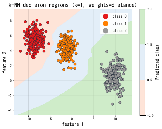
Experiments with Python #

The following Python snippet evaluates several neighbour counts on a train/validation split and plots the decision regions for the best-performing model.

from __future__ import annotations

import japanize_matplotlib
import matplotlib.pyplot as plt
import numpy as np
from matplotlib.colors import ListedColormap
from sklearn.datasets import make_blobs
from sklearn.neighbors import KNeighborsClassifier
from sklearn.pipeline import make_pipeline
from sklearn.preprocessing import StandardScaler


def run_knn_demo(
    n_samples: int = 600,
    random_state: int = 7,
    weights: str = "distance",
    k_values: tuple[int, ...] = (1, 3, 5, 7, 11),
    validation_ratio: float = 0.3,
    title: str = "k-NN decision regions",
    xlabel: str = "feature 1",
    ylabel: str = "feature 2",
    class_label_prefix: str = "class",
) -> dict[str, object]:
    """Evaluate k-NN for several neighbour counts and plot decision regions.

    Args:
        n_samples: Number of synthetic samples to draw.
        random_state: Seed for reproducible sampling.
        weights: Weighting scheme handed to KNeighborsClassifier.
        k_values: Candidate neighbour counts to evaluate.
        validation_ratio: Fraction of the data reserved for validation.
        title: Title for the generated figure.
        xlabel: Label for the x-axis.
        ylabel: Label for the y-axis.
        class_label_prefix: Prefix used when labelling the classes.

    Returns:
        Dictionary with validation scores per k and the best-performing k.
    """
    japanize_matplotlib.japanize()
    X, y = make_blobs(
        n_samples=n_samples,
        centers=3,
        cluster_std=[1.1, 1.0, 1.2],
        random_state=random_state,
    )

    rng = np.random.default_rng(random_state)
    indices = rng.permutation(len(X))
    split = int(len(X) * (1.0 - validation_ratio))
    train_idx, valid_idx = indices[:split], indices[split:]
    X_train, X_valid = X[train_idx], X[valid_idx]
    y_train, y_valid = y[train_idx], y[valid_idx]

    scores: dict[int, float] = {}
    for k in k_values:
        model = make_pipeline(
            StandardScaler(),
            KNeighborsClassifier(n_neighbors=k, weights=weights),
        )
        model.fit(X_train, y_train)
        scores[k] = float(model.score(X_valid, y_valid))

    best_k = max(scores, key=scores.get)
    best_model = make_pipeline(
        StandardScaler(),
        KNeighborsClassifier(n_neighbors=best_k, weights=weights),
    )
    best_model.fit(X, y)

    xx, yy = np.meshgrid(
        np.linspace(X[:, 0].min() - 1.5, X[:, 0].max() + 1.5, 300),
        np.linspace(X[:, 1].min() - 1.5, X[:, 1].max() + 1.5, 300),
    )
    grid = np.column_stack([xx.ravel(), yy.ravel()])
    predictions = best_model.predict(grid).reshape(xx.shape)

    unique_classes = np.unique(y)
    levels = np.arange(unique_classes.min(), unique_classes.max() + 2) - 0.5
    cmap = ListedColormap(["#fee0d2", "#deebf7", "#c7e9c0"])

    fig, ax = plt.subplots(figsize=(7, 5.5))
    contour = ax.contourf(xx, yy, predictions, levels=levels, cmap=cmap, alpha=0.85)
    scatter = ax.scatter(
        X[:, 0],
        X[:, 1],
        c=y,
        cmap="Set1",
        edgecolor="#1f2937",
        linewidth=0.6,
    )
    ax.set_title(f"{title} (k={best_k}, weights={weights})")
    ax.set_xlabel(xlabel)
    ax.set_ylabel(ylabel)
    ax.set_xlim(xx.min(), xx.max())
    ax.set_ylim(yy.min(), yy.max())
    ax.grid(alpha=0.15)

    legend = ax.legend(
        handles=scatter.legend_elements()[0],
        labels=[f"{class_label_prefix} {cls}" for cls in unique_classes],
        loc="upper right",
        frameon=True,
    )
    legend.get_frame().set_alpha(0.9)
    fig.colorbar(contour, ax=ax, label="Predicted class")
    fig.tight_layout()
    plt.show()

    return {"scores": scores, "best_k": int(best_k), "validation_accuracy": scores[best_k]}


metrics = run_knn_demo(
    title="k-NN decision regions",
    xlabel="feature 1",
    ylabel="feature 2",
    class_label_prefix="class",
)
print(f"Best k: {metrics['best_k']}")
print(f"Validation accuracy (best k): {metrics['validation_accuracy']:.3f}")
for candidate_k, score in metrics["scores"].items():
    print(f"k={candidate_k}: validation accuracy={score:.3f}")

k-NN decision regions

References #

Cover, T. M., & Hart, P. E. (1967). Nearest Neighbor Pattern Classification. IEEE Transactions on Information Theory, 13(1), 21–27.
Hastie, T., Tibshirani, R., & Friedman, J. (2009). The Elements of Statistical Learning. Springer.