Linear Discriminant Analysis (LDA)

Basic

Linear Discriminant Analysis (LDA) | Learn directions that separate classes

Created: Last updated: Read time: 3 min
まとめ
  • LDA finds directions that maximize the ratio of between-class variance to within-class variance, serving both classification and dimensionality reduction.
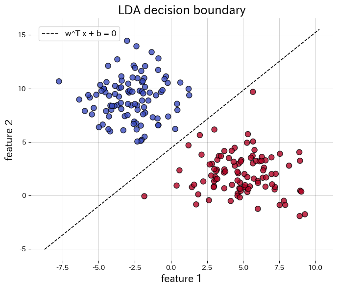
  • The decision boundary takes the form \(\mathbf{w}^\top \mathbf{x} + b = 0\), which becomes a line in 2D or a plane in 3D, giving a clear geometric interpretation.
  • Assuming each class is Gaussian with the same covariance matrix, LDA approaches the Bayes-optimal classifier.
  • scikit-learn窶冱 LinearDiscriminantAnalysis makes it easy to visualise decision boundaries and to inspect the projected features.

Intuition #

LDA searches for directions that keep samples of the same class close together while pushing samples from different classes far apart. Projecting the data onto that direction makes the classes easier to separate, so it can be used directly for classification or as a dimensionality-reduction step before another classifier.

Mathematical formulation #

For the two-class case, the projection direction \(\mathbf{w}\) maximizes

$$ J(\mathbf{w}) = \frac{\mathbf{w}^\top \mathbf{S}_B \mathbf{w}}{\mathbf{w}^\top \mathbf{S}_W \mathbf{w}}, $$

where \(\mathbf{S}_B\) is the between-class scatter matrix and \(\mathbf{S}_W\) is the within-class scatter matrix. In the multi-class case we obtain up to \(K-1\) projection directions, which can be used for dimensionality reduction.

Experiments with Python #

Below we apply LDA to a synthetic two-class data set, draw the decision boundary, and plot the projected 1D features. Calling transform returns the projected data directly.

from __future__ import annotations

import japanize_matplotlib
import matplotlib.pyplot as plt
import numpy as np
from sklearn.datasets import make_blobs
from sklearn.discriminant_analysis import LinearDiscriminantAnalysis
from sklearn.metrics import accuracy_score


def run_lda_demo(
    n_samples: int = 200,
    random_state: int = 42,
    title_boundary: str = "LDA decision boundary",
    title_projection: str = "One-dimensional projection by LDA",
    xlabel: str = "feature 1",
    ylabel: str = "feature 2",
    hist_xlabel: str = "projected feature",
    class0_label: str = "class 0",
    class1_label: str = "class 1",
) -> dict[str, float]:
    """Train LDA on synthetic blobs and plot boundary plus projection."""
    japanize_matplotlib.japanize()
    X, y = make_blobs(
        n_samples=n_samples,
        centers=2,
        n_features=2,
        cluster_std=2.0,
        random_state=random_state,
    )

    clf = LinearDiscriminantAnalysis(store_covariance=True)
    clf.fit(X, y)

    accuracy = float(accuracy_score(y, clf.predict(X)))
    w = clf.coef_[0]
    b = float(clf.intercept_[0])

    xs = np.linspace(X[:, 0].min() - 1, X[:, 0].max() + 1, 300)
    ys_boundary = -(w[0] / w[1]) * xs - b / w[1]

    fig, ax = plt.subplots(figsize=(7, 6))
    ax.set_title(title_boundary)
    ax.scatter(X[:, 0], X[:, 1], c=y, cmap="coolwarm", edgecolor="k", alpha=0.8)
    ax.plot(xs, ys_boundary, "k--", lw=1.2, label="w^T x + b = 0")
    ax.set_xlabel(xlabel)
    ax.set_ylabel(ylabel)
    ax.legend(loc="best")
    ax.grid(alpha=0.25)
    fig.tight_layout()
    plt.show()

    X_proj = clf.transform(X)[:, 0]

    fig, ax = plt.subplots(figsize=(8, 4))
    ax.set_title(title_projection)
    ax.hist(X_proj[y == 0], bins=20, alpha=0.7, label=class0_label)
    ax.hist(X_proj[y == 1], bins=20, alpha=0.7, label=class1_label)
    ax.set_xlabel(hist_xlabel)
    ax.legend(loc="best")
    ax.grid(alpha=0.25)
    fig.tight_layout()
    plt.show()

    return {"accuracy": accuracy}


metrics = run_lda_demo(
    title_boundary="LDA decision boundary",
    title_projection="One-dimensional projection by LDA",
    xlabel="feature 1",
    ylabel="feature 2",
    hist_xlabel="projected feature",
    class0_label="class 0",
    class1_label="class 1",
)
print(f"Training accuracy: {metrics['accuracy']:.3f}")

Calling transform returns the projected data directly figure

References #

  • Fisher, R. A. (1936). The Use of Multiple Measurements in Taxonomic Problems. Annals of Eugenics, 7(2), 179窶・88.
  • Hastie, T., Tibshirani, R., & Friedman, J. (2009). The Elements of Statistical Learning. Springer.