Perceptron | K

まとめ

The perceptron converges in a finite number of updates on linearly separable data, making it one of the oldest classification algorithms.
Predictions use the sign of a weighted sum $\mathbf{w}^\top \mathbf{x} + b$; if the sign is wrong, the corresponding sample updates the weights.
The update rule窶蚤dding the misclassified sample scaled by the learning rate窶廃rovides an intuitive introduction to gradient-based methods.
When data are not linearly separable, feature expansion or kernel tricks are needed.

Intuition #

The perceptron moves the decision boundary whenever it misclassifies a sample, nudging it toward the correct side. The weight vector $\mathbf{w}$ is normal to the decision boundary, while the bias $b$ controls the offset. A learning rate $\eta$ determines how large each nudge should be.

Mathematical formulation #

Predictions are computed as

$$ \hat{y} = \operatorname{sign}(\mathbf{w}^\top \mathbf{x} + b). $$

If a sample $(\mathbf{x}_i, y_i)$ is misclassified, update the parameters via

$$ \mathbf{w} \leftarrow \mathbf{w} + \eta, y_i, \mathbf{x}_i,\qquad b \leftarrow b + \eta, y_i. $$

When the data are linearly separable, this procedure is guaranteed to converge.

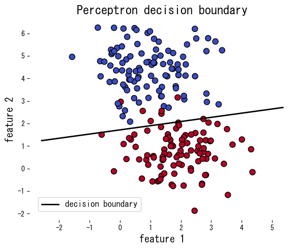
Experiments with Python #

The following example applies the perceptron to synthetic data, reporting the number of mistakes per epoch and plotting the resulting decision boundary.

from __future__ import annotations

import japanize_matplotlib
import matplotlib.pyplot as plt
import numpy as np
from sklearn.datasets import make_blobs
from sklearn.metrics import accuracy_score


def run_perceptron_demo(
    n_samples: int = 200,
    lr: float = 0.1,
    n_epochs: int = 20,
    random_state: int = 0,
    title: str = "Perceptron decision boundary",
    xlabel: str = "feature 1",
    ylabel: str = "feature 2",
    label_boundary: str = "decision boundary",
) -> dict[str, object]:
    """Train a perceptron on synthetic blobs and plot the decision boundary."""
    japanize_matplotlib.japanize()
    X, y = make_blobs(n_samples=n_samples, centers=2, cluster_std=1.0, random_state=random_state)
    y_signed = np.where(y == 0, -1, 1)

    w = np.zeros(X.shape[1])
    b = 0.0
    history: list[int] = []

    for _ in range(n_epochs):
        errors = 0
        for xi, target in zip(X, y_signed):
            update = lr * target if target * (np.dot(w, xi) + b) <= 0 else 0.0
            if update != 0.0:
                w += update * xi
                b += update
                errors += 1
        history.append(int(errors))
        if errors == 0:
            break

    preds = np.where(np.dot(X, w) + b >= 0, 1, -1)
    accuracy = float(accuracy_score(y_signed, preds))

    xx = np.linspace(X[:, 0].min() - 1, X[:, 0].max() + 1, 200)
    yy = -(w[0] * xx + b) / w[1]

    fig, ax = plt.subplots(figsize=(6, 5))
    ax.scatter(X[:, 0], X[:, 1], c=y, cmap="coolwarm", edgecolor="k")
    ax.plot(xx, yy, color="black", linewidth=2, label=label_boundary)
    ax.set_xlabel(xlabel)
    ax.set_ylabel(ylabel)
    ax.set_title(title)
    ax.legend(loc="best")
    fig.tight_layout()
    plt.show()

    return {"weights": w, "bias": b, "errors": history, "accuracy": accuracy}


metrics = run_perceptron_demo(
    title="Perceptron decision boundary",
    xlabel="feature 1",
    ylabel="feature 2",
    label_boundary="decision boundary",
)
print(f"Training accuracy: {metrics['accuracy']:.3f}")
print("Weights:", metrics['weights'])
print(f"Bias: {metrics['bias']:.3f}")
print("Errors per epoch:", metrics['errors'])

perceptron block 1

References #

Rosenblatt, F. (1958). The Perceptron: A Probabilistic Model for Information Storage and Organization in the Brain. Psychological Review, 65(6), 386窶・08.
Goodfellow, I., Bengio, Y., & Courville, A. (2016). Deep Learning. MIT Press.