- Softmax regression generalises logistic regression to multiple classes, producing the probability of every class simultaneously.
- Outputs lie in \([0, 1]\) and sum to 1, so they plug directly into decision thresholds, cost-sensitive rules, or downstream pipelines.
- Training minimises the cross-entropy loss, directly correcting discrepancies between predicted and true probability distributions.
- In scikit-learn,
LogisticRegression(multi_class="multinomial")implements softmax regression and supports L1/L2 regularisation.
Intuition #
In the binary case the sigmoid provides the probability of class 1. With multiple classes we want all probabilities together. Softmax regression takes a linear score for each class, exponentiates the scores, and normalises them so they form a valid probability distribution. Higher scores become emphasised while lower scores are suppressed.
Mathematical formulation #
Let \(K\) be the number of classes, \(\mathbf{w}_k\) and \(b_k\) the parameters for class \(k\). Then
$$ P(y = k \mid \mathbf{x}) = \frac{\exp\left(\mathbf{w}k^\top \mathbf{x} + b_k\right)} {\sum{j=1}^{K} \exp\left(\mathbf{w}_j^\top \mathbf{x} + b_j\right)}. $$
The objective is the cross-entropy loss
$$ L = - \sum_{i=1}^{n} \sum_{k=1}^{K} \mathbb{1}(y_i = k) \log P(y = k \mid \mathbf{x}_i), $$
with optional regularisation on the weights to prevent overfitting.
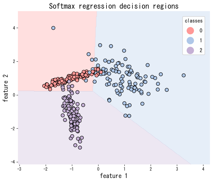
Experiments with Python #
The script below applies softmax regression to a synthetic three-class data set and visualises the decision regions. Setting multi_class="multinomial" activates the softmax formulation.
from __future__ import annotations
import japanize_matplotlib
import matplotlib.pyplot as plt
import numpy as np
from matplotlib.colors import ListedColormap
from sklearn.datasets import make_classification
from sklearn.linear_model import LogisticRegression
from sklearn.metrics import accuracy_score
def run_softmax_regression_demo(
n_samples: int = 300,
n_classes: int = 3,
random_state: int = 42,
label_title: str = "Softmax regression decision regions",
xlabel: str = "feature 1",
ylabel: str = "feature 2",
) -> dict[str, float]:
"""Train a softmax regression model and visualise decision regions."""
japanize_matplotlib.japanize()
X, y = make_classification(
n_samples=n_samples,
n_features=2,
n_informative=2,
n_redundant=0,
n_clusters_per_class=1,
n_classes=n_classes,
random_state=random_state,
)
clf = LogisticRegression(multi_class="multinomial", solver="lbfgs")
clf.fit(X, y)
accuracy = float(accuracy_score(y, clf.predict(X)))
x1_min, x1_max = X[:, 0].min() - 1.0, X[:, 0].max() + 1.0
x2_min, x2_max = X[:, 1].min() - 1.0, X[:, 1].max() + 1.0
grid_x1, grid_x2 = np.meshgrid(
np.linspace(x1_min, x1_max, 400),
np.linspace(x2_min, x2_max, 400),
)
grid_points = np.c_[grid_x1.ravel(), grid_x2.ravel()]
preds = clf.predict(grid_points).reshape(grid_x1.shape)
cmap = ListedColormap(["#ff9896", "#98df8a", "#aec7e8", "#f7b6d2", "#c5b0d5"])
fig, ax = plt.subplots(figsize=(7, 6))
ax.contourf(grid_x1, grid_x2, preds, alpha=0.3, cmap=cmap, levels=np.arange(-0.5, n_classes + 0.5, 1))
scatter = ax.scatter(X[:, 0], X[:, 1], c=y, edgecolor="k", cmap=cmap)
ax.set_xlabel(xlabel)
ax.set_ylabel(ylabel)
ax.set_title(label_title)
legend = ax.legend(*scatter.legend_elements(), title="classes", loc="best")
ax.add_artist(legend)
fig.tight_layout()
plt.show()
return {"accuracy": accuracy}
metrics = run_softmax_regression_demo(
label_title="Softmax regression decision regions",
xlabel="feature 1",
ylabel="feature 2",
)
print(f"Training accuracy: {metrics['accuracy']:.3f}")

References #
- Bishop, C. M. (2006). Pattern Recognition and Machine Learning. Springer.
- Murphy, K. P. (2012). Machine Learning: A Probabilistic Perspective. MIT Press.