Support Vector Machines (SVM)

まとめ

SVM learns a decision boundary that maximises the margin between classes, emphasising generalisation.
Soft margins introduce slack variables so that some misclassifications are allowed while the penalty $C$ balances margin width and errors.
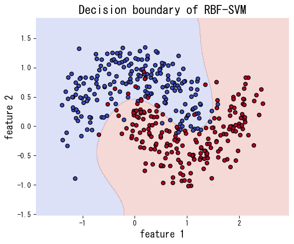
Kernel tricks replace dot products with kernel functions, enabling non-linear decision boundaries without explicit feature expansion.
Feature standardisation and hyperparameter tuning (e.g. $C$, $\gamma$) are crucial for good performance.

Intuition #

Among all separating hyperplanes, SVM picks the one that leaves the widest margin to the training samples. Points that touch the margin are the support vectors; only they determine the final boundary. As a result, the classifier is resilient to modest noise.

Mathematical formulation #

For linearly separable data we solve

$$ \min_{\mathbf{w}, b} \ \frac{1}{2} \lVert \mathbf{w} \rVert_2^2 \quad \text{s.t.} \quad y_i(\mathbf{w}^\top \mathbf{x}_i + b) \ge 1. $$

In practice we use the soft-margin variant with slack variables $\xi_i \ge 0$:

$$ \min_{\mathbf{w}, b, \boldsymbol{\xi}} \ \frac{1}{2} \lVert \mathbf{w} \rVert_2^2 + C \sum_{i=1}^{n} \xi_i \quad \text{s.t.} \quad y_i(\mathbf{w}^\top \mathbf{x}_i + b) \ge 1 - \xi_i. $$

Replacing inner products $\mathbf{x}_i^\top \mathbf{x}_j$ with kernels $K(\mathbf{x}_i, \mathbf{x}_j)$ yields non-linear decision boundaries.

Experiments with Python #

The code below fits SVM with a linear kernel and with an RBF kernel on a non-linearly separable data set generated by make_moons. The RBF kernel captures the curved boundary much better.

from __future__ import annotations

import japanize_matplotlib
import matplotlib.pyplot as plt
import numpy as np
from sklearn.datasets import make_moons
from sklearn.metrics import accuracy_score
from sklearn.pipeline import make_pipeline
from sklearn.preprocessing import StandardScaler
from sklearn.svm import SVC


def run_svm_demo(
    n_samples: int = 400,
    noise: float = 0.25,
    random_state: int = 42,
    title: str = "Decision boundary of RBF-SVM",
    xlabel: str = "feature 1",
    ylabel: str = "feature 2",
) -> dict[str, float]:
    """Train linear and RBF SVMs and plot the RBF decision boundary."""
    japanize_matplotlib.japanize()
    X, y = make_moons(n_samples=n_samples, noise=noise, random_state=random_state)

    linear_clf = make_pipeline(StandardScaler(), SVC(kernel="linear", C=1.0))
    linear_clf.fit(X, y)

    rbf_clf = make_pipeline(StandardScaler(), SVC(kernel="rbf", C=5.0, gamma=0.5))
    rbf_clf.fit(X, y)

    linear_acc = float(accuracy_score(y, linear_clf.predict(X)))
    rbf_acc = float(accuracy_score(y, rbf_clf.predict(X)))

    grid_x, grid_y = np.meshgrid(
        np.linspace(X[:, 0].min() - 0.5, X[:, 0].max() + 0.5, 400),
        np.linspace(X[:, 1].min() - 0.5, X[:, 1].max() + 0.5, 400),
    )
    grid = np.c_[grid_x.ravel(), grid_y.ravel()]
    rbf_scores = rbf_clf.predict(grid).reshape(grid_x.shape)

    fig, ax = plt.subplots(figsize=(6, 5))
    ax.contourf(grid_x, grid_y, rbf_scores, alpha=0.2, cmap="coolwarm")
    ax.scatter(X[:, 0], X[:, 1], c=y, cmap="coolwarm", edgecolor="k", s=30)
    ax.set_title(title)
    ax.set_xlabel(xlabel)
    ax.set_ylabel(ylabel)
    fig.tight_layout()
    plt.show()

    return {"linear_accuracy": linear_acc, "rbf_accuracy": rbf_acc}


metrics = run_svm_demo(
    title="Decision boundary of RBF-SVM",
    xlabel="feature 1",
    ylabel="feature 2",
)
print(f"Linear kernel accuracy: {metrics['linear_accuracy']:.3f}")
print(f"RBF kernel accuracy: {metrics['rbf_accuracy']:.3f}")

svm block 1

References #

Vapnik, V. (1998). Statistical Learning Theory. Wiley.
Smola, A. J., & Schﾃｶlkopf, B. (2004). A Tutorial on Support Vector Regression. Statistics and Computing, 14(3), 199窶・22.