DBSCAN

Intuition #

This method should be interpreted through its assumptions, data conditions, and how parameter choices affect generalization.

Detailed Explanation #

1. Overview #

DBSCAN does not require the number of clusters beforehand. Instead, it inspects each sample:

• Core points: at least min_samples neighbours within distance eps.
• Border points: lie within the eps-ball of a core point but fail the core criterion themselves.
• Noise points: belong to no core neighbourhood.

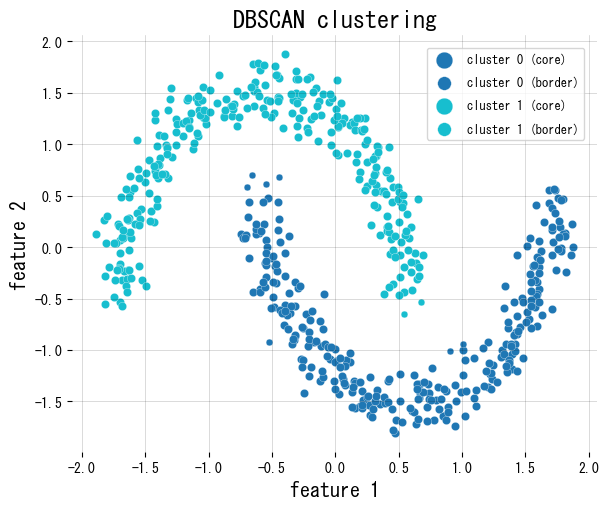
Because of this density view, DBSCAN is robust to non-convex clusters such as two moons or concentric circles. Always scale the features so eps has a meaningful interpretation.

2. Formal definition #

Given (x_i \in \mathcal{X}), its (\varepsilon)-neighbourhood is

If (|\mathcal{N}_\varepsilon(x_i)| \ge \texttt{min_samples}|), the point is core. DBSCAN builds clusters by exploring density-reachable points; anything left unvisited becomes noise. With a spatial index the overall complexity is (O(n \log n)).

3. Python example #

The snippet below uses scikit-learn’s DBSCAN on a two-moons dataset, colours core/border points differently, and reports how many samples are marked as noise.

 1
 2
 3
 4
 5
 6
 7
 8
 9
10
11
12
13
14
15
16
17
18
19
20
21
22
23
24
25
26
27
28
29
30
31
32
33
34
35
36
37
38
39
40
41
42
43
44
45
46
47
48
49
50
51
52
53
54
55
56
57
58
59
60
61
62
63
64
65
66
67
68
69
70
71
72
73
74
75
76
77
78
79
80
81
82
83
84
85
86
87

from __future__ import annotations

import japanize_matplotlib
import matplotlib.pyplot as plt
import numpy as np
from numpy.typing import NDArray
from sklearn.cluster import DBSCAN
from sklearn.datasets import make_moons
from sklearn.preprocessing import StandardScaler

def run_dbscan_demo(
    n_samples: int = 600,
    noise: float = 0.08,
    eps: float = 0.3,
    min_samples: int = 10,
    random_state: int = 0,
) -> dict[str, int]:
    japanize_matplotlib.japanize()
    features, _ = make_moons(
        n_samples=n_samples,
        noise=noise,
        random_state=random_state,
    )
    features = StandardScaler().fit_transform(features)

    model = DBSCAN(eps=eps, min_samples=min_samples)
    labels = model.fit_predict(features)

    unique_labels = sorted(np.unique(labels))
    cluster_ids = [label for label in unique_labels if label != -1]
    noise_count = int(np.sum(labels == -1))

    core_mask = np.zeros(labels.shape[0], dtype=bool)
    if hasattr(model, "core_sample_indices_"):
        core_mask[model.core_sample_indices_] = True

    fig, ax = plt.subplots(figsize=(6.2, 5.2))
    palette = plt.cm.get_cmap("tab10", max(len(cluster_ids), 1))

    for order, cluster_id in enumerate(cluster_ids):
        mask = labels == cluster_id
        color = palette(order)
        ax.scatter(
            features[mask & core_mask, 0],
            features[mask & core_mask, 1],
            c=[color],
            s=36,
            edgecolor="white",
            linewidth=0.2,
            label=f"Cluster {cluster_id} core",
        )
        ax.scatter(
            features[mask & ~core_mask, 0],
            features[mask & ~core_mask, 1],
            c=[color],
            s=24,
            edgecolor="white",
            linewidth=0.2,
            marker="o",
            label=f"Cluster {cluster_id} border",
        )

    if noise_count:
        noise_mask = labels == -1
        ax.scatter(
            features[noise_mask, 0],
            features[noise_mask, 1],
            c="#9ca3af",
            marker="x",
            s=28,
            linewidth=0.8,
            label="Noise",
        )

    ax.set_title("DBSCAN clustering demo")
    ax.set_xlabel("Feature 1")
    ax.set_ylabel("Feature 2")
    ax.grid(alpha=0.2)
    ax.legend(loc="upper right", fontsize=9)
    fig.tight_layout()
    plt.show()

    return {"n_clusters": len(cluster_ids), "n_noise": noise_count}

result = run_dbscan_demo()
print(f"Clusters discovered: {result['n_clusters']}")
print(f"Noise points: {result['n_noise']}")

4. Practical tips #

• Plot the sorted distances to the k-th neighbour (k = min_samples) to pick eps where the curve exhibits an elbow.
• Use pipelines so standardisation and clustering run together; otherwise distance-based decisions become meaningless.
• For very large datasets consider approximate nearest neighbours or switch to HDBSCAN, which extends DBSCAN to multi-density data and removes the need to tune eps.

FAQ #

What is DBSCAN? #

DBSCAN (Density-Based Spatial Clustering of Applications with Noise) is an unsupervised clustering algorithm that groups points based on local density rather than distance to a centroid. It discovers clusters of arbitrary shape and automatically marks low-density points as noise (label -1), without requiring you to specify the number of clusters in advance.

What are the two main parameters of DBSCAN? #

• eps (ε): the radius that defines a point’s neighbourhood. Two points are neighbours if their distance is ≤ ε.
• min_samples: the minimum number of neighbours within ε for a point to be considered a core point. Larger values create denser, smaller clusters and more noise.

A practical tuning recipe: fix min_samples to dimensionality + 1 (or higher for noisy data), then plot the sorted distance to the k-th nearest neighbour and pick ε at the “elbow” of the curve.

How does DBSCAN differ from k-means? #

Use k-means for compact, well-separated blobs; use DBSCAN when clusters have irregular shapes or you expect noise/outliers.

Why do I need to scale features before DBSCAN? #

DBSCAN uses a distance threshold eps to define neighbourhoods. If features have vastly different scales (e.g., age in years vs. income in thousands), the distance calculation will be dominated by the high-scale feature, making eps meaningless. Always apply StandardScaler or MinMaxScaler before fitting.

When should I use HDBSCAN instead of DBSCAN? #

Choose HDBSCAN when:

• Your dataset has clusters of varying density (DBSCAN’s single eps cannot handle this).
• You want to avoid tuning eps (HDBSCAN only needs min_cluster_size).
• You want a more stable solution across different datasets.

HDBSCAN builds a full density hierarchy and extracts the most persistent clusters, making it more robust than DBSCAN for real-world data.

5. References #