Adaboost(Regression)

Last updated 2026-03-04 Read time 3 min

Summary

AdaBoost regression (AdaBoost.R2) improves predictions by reweighting samples with larger residual errors.
Weight updates depend on the error profile, so noise and outliers directly affect the final ensemble.
Cross-validating n_estimators and learning_rate is essential to balance fit quality and generalization.

Intuition #

AdaBoost regression repeatedly emphasizes regions where current predictors perform poorly. By reallocating attention to high-error samples, the ensemble captures nonlinear residual patterns that single learners often miss.

Detailed Explanation #

1
2
3
4
5
import numpy as np
import matplotlib.pyplot as plt
import japanize_matplotlib
from sklearn.tree import DecisionTreeRegressor
from sklearn.ensemble import AdaBoostRegressor

 1
 2
 3
 4
 5
 6
 7
 8
 9
10
11
12
13
14
15
16
17
18
19
20
21
22
23
24
25
26
27
# NOTE: This model is to check the model's sample_weight
class DummyRegressor:
    def __init__(self):
        self.model = DecisionTreeRegressor(max_depth=5)
        self.error_vector = None
        self.X_for_plot = None
        self.y_for_plot = None

    def fit(self, X, y):
        self.model.fit(X, y)
        y_pred = self.model.predict(X)

        # Weights are calculated based on regression error.
        # https://github.com/scikit-learn/scikit-learn/blob/main/sklearn/ensemble/_weight_boosting.py#L1130
        self.error_vector = np.abs(y_pred - y)
        self.X_for_plot = X.copy()
        self.y_for_plot = y.copy()
        return self.model

    def predict(self, X, check_input=True):
        return self.model.predict(X)

    def get_params(self, deep=False):
        return {}

    def set_params(self, deep=False):
        return {}

Fit regression models to training data #

 1
 2
 3
 4
 5
 6
 7
 8
 9
10
11
12
13
14
15
16
17
18
19
20
21
22
23
# training dataset
X = np.linspace(-10, 10, 500)[:, np.newaxis]
y = (np.sin(X).ravel() + np.cos(4 * X).ravel()) * 10 + 10 + np.linspace(-2, 2, 500)

## train Adaboost regressor
reg = AdaBoostRegressor(
    DummyRegressor(),
    n_estimators=100,
    random_state=100,
    loss="linear",
    learning_rate=0.8,
)
reg.fit(X, y)
y_pred = reg.predict(X)

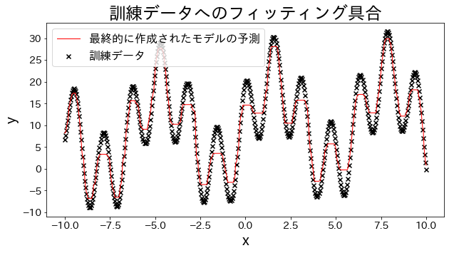
# Check the fitting to the training data.
plt.figure(figsize=(10, 5))
plt.scatter(X, y, c="k", marker="x", label="訓練データ")
plt.plot(X, y_pred, c="r", label="prediction", linewidth=1)
plt.xlabel("x")
plt.ylabel("y")
plt.legend()
plt.show()

png

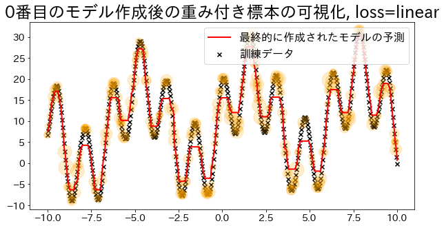
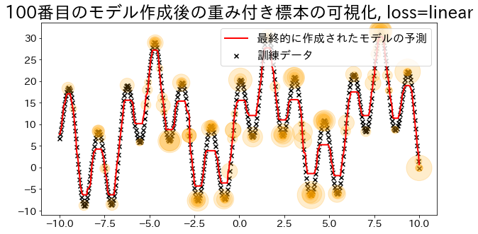
Visualize sample weights (for loss=‘linear’) #

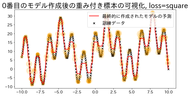
Adaboost determines the weights based on the errors of the regression. Visualize the magnitude of the weights when specified as ’linear’. Observe how data with added weights have a higher probability of being sampled during training.

loss{‘linear’, ‘square’, ‘exponential’}, default=’linear’ The loss function to use when updating the weights after each boosting iteration.

sklearn.ensemble.AdaBoostRegressor

 1
 2
 3
 4
 5
 6
 7
 8
 9
10
11
12
13
14
15
16
17
18
19
20
21
22
23
24
25
26
27
28
29
30
31
32
33
34
35
36
37
38
39
40
41
42
43
44
45
46
47
48
49
50
51
52
53
54
def visualize_weight(reg, X, y, y_pred):
    """Function for plotting the value (number of times sampled) corresponding to the weights of the sample

    Parameters
    ----------
    reg : sklearn.ensemble._weight_boosting
        boosting model
    X : numpy.ndarray
        training dataset
    y : numpy.ndarray
        target
    y_pred:
        prediction
    """
    assert reg.estimators_ is not None, "len(reg.estimators_) > 0"

    for i, estimators_i in enumerate(reg.estimators_):
        if i % 100 == 0:
            # Count how many times the data appears in the data used to create the i-th model
            weight_dict = {xi: 0 for xi in X.ravel()}
            for xi in estimators_i.X_for_plot.ravel():
                weight_dict[xi] += 1

            # Plot the number of occurrences as orange circles on the graph (the more the number, the larger the circle)
            weight_x_sorted = sorted(weight_dict.items(), key=lambda x: x[0])
            weight_vec = np.array([s * 100 for xi, s in weight_x_sorted])

            # plot graph
            plt.figure(figsize=(10, 5))
            plt.title(f"Visualization of the weighted sample after creating the {i}-th model, loss={reg.loss}")
            plt.scatter(X, y, c="k", marker="x", label="training data")
            plt.scatter(
                estimators_i.X_for_plot,
                estimators_i.y_for_plot,
                marker="o",
                alpha=0.2,
                c="orange",
                s=weight_vec,
            )
            plt.plot(X, y_pred, c="r", label="prediction", linewidth=2)
            plt.legend(loc="upper right")
            plt.show()

## Create a regression model with loss="linear
reg = AdaBoostRegressor(
    DummyRegressor(),
    n_estimators=101,
    random_state=100,
    loss="linear",
    learning_rate=1,
)
reg.fit(X, y)
y_pred = reg.predict(X)
visualize_weight(reg, X, y, y_pred)

png

 1
 2
 3
 4
 5
 6
 7
 8
 9
10
11
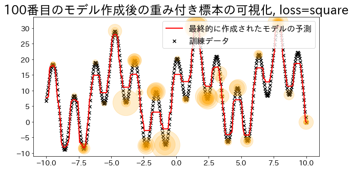
## Create regression model with loss="square
reg = AdaBoostRegressor(
    DummyRegressor(),
    n_estimators=101,
    random_state=100,
    loss="square",
    learning_rate=1,
)
reg.fit(X, y)
y_pred = reg.predict(X)
visualize_weight(reg, X, y, y_pred)

png