Gradient boosting

Last updated 2026-03-04 Read time 4 min

Summary

Gradient Boosting builds an additive model by fitting each new weak learner to the current residual signal.
learning_rate and n_estimators jointly control optimization speed and overfitting risk.
The loss function choice changes robustness to outliers and the shape of the fitted function.

Intuition #

Gradient Boosting starts with a rough prediction, then repeatedly adds small trees that correct what the current model still gets wrong. Many small, targeted corrections accumulate into a flexible predictor.

Detailed Explanation #

1
2
3
4
import numpy as np
import matplotlib.pyplot as plt
import japanize_matplotlib
from sklearn.ensemble import GradientBoostingRegressor

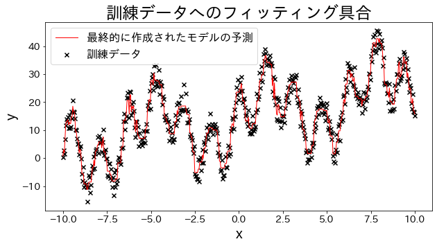
Fit a regression model to training data #

Create experimental data, waveform data with trigonometric functions added together.

 1
 2
 3
 4
 5
 6
 7
 8
 9
10
11
12
13
14
15
16
17
18
19
20
21
22
23
24
25
26
27
28
29
# training dataset
X = np.linspace(-10, 10, 500)[:, np.newaxis]
noise = np.random.rand(X.shape[0]) * 10

# target
y = (
    (np.sin(X).ravel() + np.cos(4 * X).ravel()) * 10
    + 10
    + np.linspace(-10, 10, 500)
    + noise
)

# train gradient boosting
reg = GradientBoostingRegressor(
    n_estimators=50,
    learning_rate=0.5,
)
reg.fit(X, y)
y_pred = reg.predict(X)

# Check the fitting to the training data
plt.figure(figsize=(10, 5))
plt.scatter(X, y, c="k", marker="x", label="training data")
plt.plot(X, y_pred, c="r", label="Predictions for the final created model", linewidth=1)
plt.xlabel("x")
plt.ylabel("y")
plt.title("Degree of fitting to training dataset")
plt.legend()
plt.show()

png

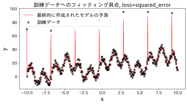
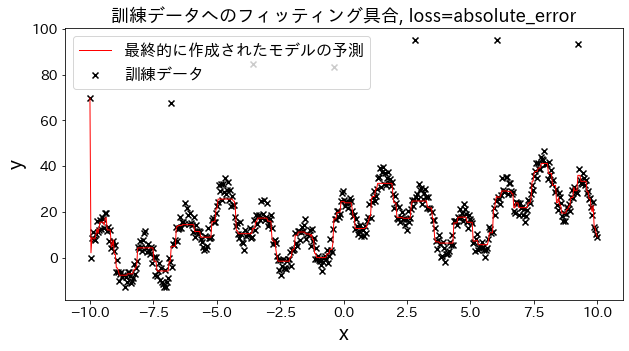
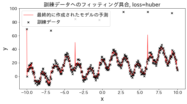
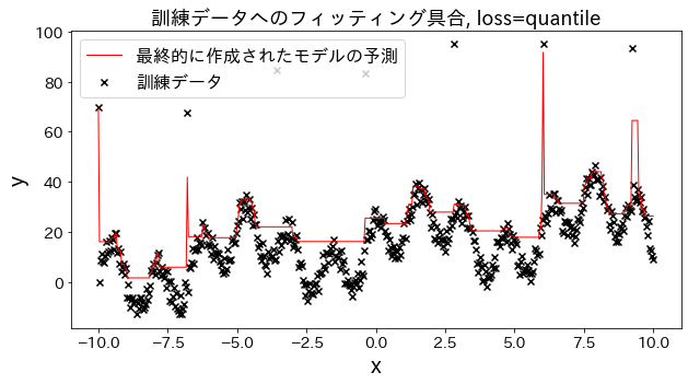
Effect of loss function on results #

Check how fitting to the training data changes when loss is changed to [“squared_error”, “absolute_error”, “huber”, “quantile”]." It is expected that “absolute_error” and “huber” will not go on to predict outliers since the penalty for outliers is not as large as the squared error.

 1
 2
 3
 4
 5
 6
 7
 8
 9
10
11
12
13
14
15
16
17
18
19
20
21
22
23
24
25
26
27
28
29
30
31
32
33
34
35
36
# training data
X = np.linspace(-10, 10, 500)[:, np.newaxis]

# prepare outliers
noise = np.random.rand(X.shape[0]) * 10
for i, ni in enumerate(noise):
    if i % 80 == 0:
        noise[i] = 70 + np.random.randint(-10, 10)

# target
y = (
    (np.sin(X).ravel() + np.cos(4 * X).ravel()) * 10
    + 10
    + np.linspace(-10, 10, 500)
    + noise
)

for loss in ["squared_error", "absolute_error", "huber", "quantile"]:
    # train gradient boosting
    reg = GradientBoostingRegressor(
        n_estimators=50,
        learning_rate=0.5,
        loss=loss,
    )
    reg.fit(X, y)
    y_pred = reg.predict(X)

    # Check the fitting to the training data.
    plt.figure(figsize=(10, 5))
    plt.scatter(X, y, c="k", marker="x", label="training dataset")
    plt.plot(X, y_pred, c="r", label="Predictions for the final created model", linewidth=1)
    plt.xlabel("x")
    plt.ylabel("y")
    plt.title(f"Degree of fitting to training data, loss={loss}", fontsize=18)
    plt.legend()
    plt.show()

png

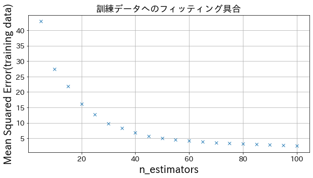
Effect of `n_estimators` on results #

You can see how the degree of improvement comes to a head when you increase n_estimators to some extent.

 1
 2
 3
 4
 5
 6
 7
 8
 9
10
11
12
13
14
15
16
17
18
19
20
21
22
23
24
25
26
27
28
29
30
31
32
33
from sklearn.metrics import mean_squared_error as MSE

# trainig dataset
X = np.linspace(-10, 10, 500)[:, np.newaxis]
noise = np.random.rand(X.shape[0]) * 10

# target
y = (
    (np.sin(X).ravel() + np.cos(4 * X).ravel()) * 10
    + 10
    + np.linspace(-10, 10, 500)
    + noise
)

# Try to create a model with different n_estimators
n_estimators_list = [(i + 1) * 5 for i in range(20)]
mses = []
for n_estimators in n_estimators_list:
    reg = GradientBoostingRegressor(
        n_estimators=n_estimators,
        learning_rate=0.3,
    )
    reg.fit(X, y)
    y_pred = reg.predict(X)
    mses.append(MSE(y, y_pred))

# Plotting mean_squared_error for different n_estimators
plt.figure(figsize=(10, 5))
plt.plot(n_estimators_list, mses, "x")
plt.xlabel("n_estimators")
plt.ylabel("Mean Squared Error(training data)")
plt.grid()
plt.show()

png

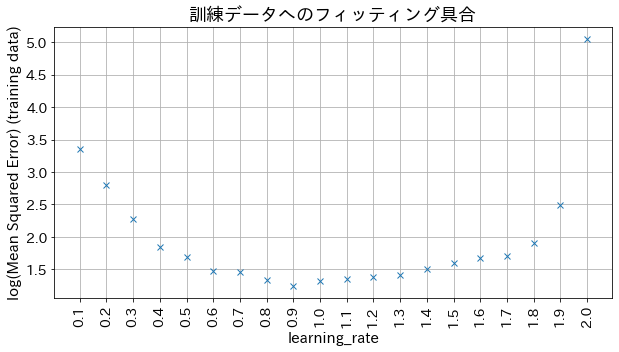
Impact of learning_rate on results #

If learning_rate is too small, the accuracy does not improve, and if learning_rate is too large, it does not converge.

 1
 2
 3
 4
 5
 6
 7
 8
 9
10
11
12
13
14
15
16
17
18
19
20
21
# Try to create a model with different n_estimators
learning_rate_list = [np.round(0.1 * (i + 1), 1) for i in range(20)]
mses = []
for learning_rate in learning_rate_list:
    reg = GradientBoostingRegressor(
        n_estimators=30,
        learning_rate=learning_rate,
    )
    reg.fit(X, y)
    y_pred = reg.predict(X)
    mses.append(np.log(MSE(y, y_pred)))

# Plotting mean_squared_error for different n_estimators
plt.figure(figsize=(10, 5))
plt_index = [i for i in range(len(learning_rate_list))]
plt.plot(plt_index, mses, "x")
plt.xticks(plt_index, learning_rate_list, rotation=90)
plt.xlabel("learning_rate", fontsize=15)
plt.ylabel("log(Mean Squared Error) (training data)", fontsize=15)
plt.grid()
plt.show()

png