Summary- Random Forest combines bootstrap sampling with random feature subsets to build diverse decision trees.
- Aggregating many decorrelated trees reduces variance and usually improves out-of-sample performance.
- Hyperparameters such as
n_estimators, max_features, and tree depth determine the balance between bias, variance, and runtime.
Intuition
#
Random Forest is bagging plus feature randomness at each split. Because trees are forced to look at different subsets of predictors, they become less correlated, and averaging them gives a stronger and more robust final model.
Detailed Explanation
#
1
2
| import numpy as np
import matplotlib.pyplot as plt
|
Train Random Forests
#
For ROC-AUC, see ROC-AUC for an explanation of how to plot.
 1
 2
 3
 4
 5
 6
 7
 8
 9
10
11
12
13
14
15
16
17
18
19
20
21
22
23
24
25
26
| from sklearn.datasets import make_classification
from sklearn.ensemble import RandomForestClassifier
from sklearn.model_selection import train_test_split
from sklearn.metrics import roc_auc_score
n_features = 20
X, y = make_classification(
n_samples=2500,
n_features=n_features,
n_informative=10,
n_classes=2,
n_redundant=0,
n_clusters_per_class=4,
random_state=777,
)
X_train, X_test, y_train, y_test = train_test_split(
X, y, test_size=0.33, random_state=777
)
model = RandomForestClassifier(
n_estimators=50, max_depth=3, random_state=777, bootstrap=True, oob_score=True
)
model.fit(X_train, y_train)
y_pred = model.predict(X_test)
rf_score = roc_auc_score(y_test, y_pred)
print(f"ROC-AUC @ test dataset = {rf_score}")
|
ROC-AUC @ test dataset = 0.814573097628059
 1
 2
 3
 4
 5
 6
 7
 8
 9
10
11
12
13
14
15
16
| import japanize_matplotlib
estimator_scores = []
for i in range(10):
estimator = model.estimators_[i]
estimator_pred = estimator.predict(X_test)
estimator_scores.append(roc_auc_score(y_test, estimator_pred))
plt.figure(figsize=(10, 4))
bar_index = [i for i in range(len(estimator_scores))]
plt.bar(bar_index, estimator_scores)
plt.bar([10], rf_score)
plt.xticks(bar_index + [10], bar_index + ["RF"])
plt.xlabel("tree index")
plt.ylabel("ROC-AUC")
plt.show()
|
Feature Importance
#
Importance based on impurity
#
1
2
3
4
5
6
| plt.figure(figsize=(10, 4))
feature_index = [i for i in range(n_features)]
plt.bar(feature_index, model.feature_importances_)
plt.xlabel("Feature Index")
plt.ylabel("Feature Importance")
plt.show()
|
permutation importance
#
 1
 2
 3
 4
 5
 6
 7
 8
 9
10
11
| from sklearn.inspection import permutation_importance
p_imp = permutation_importance(
model, X_train, y_train, n_repeats=10, random_state=77
).importances_mean
plt.figure(figsize=(10, 4))
plt.bar(feature_index, p_imp)
plt.xlabel("Feature Index")
plt.ylabel("Feature Importance")
plt.show()
|
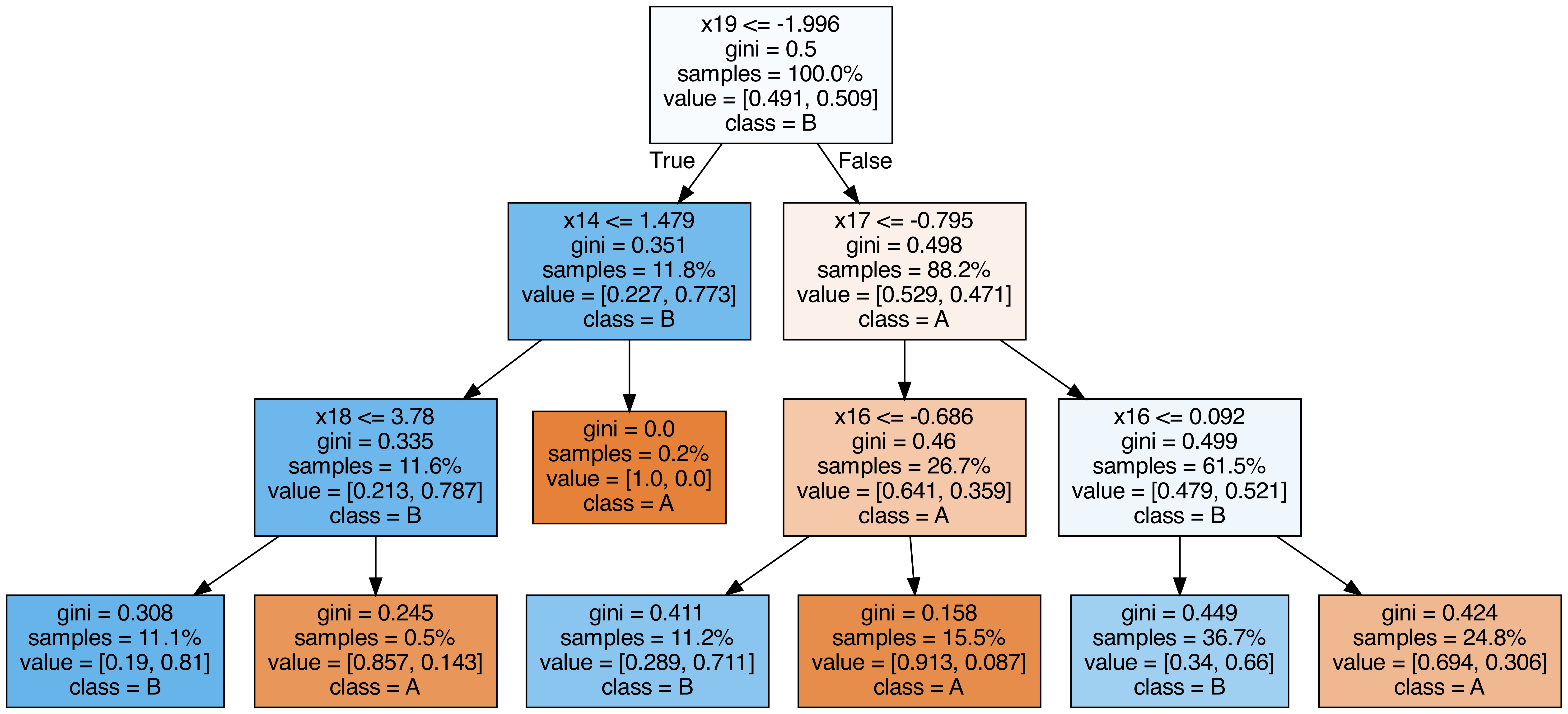
Output each tree contained in the random forest
#
 1
 2
 3
 4
 5
 6
 7
 8
 9
10
11
12
13
14
15
16
17
18
19
20
21
22
| from sklearn.tree import export_graphviz
from subprocess import call
from IPython.display import Image
from IPython.display import display
for i in range(10):
try:
estimator = model.estimators_[i]
export_graphviz(
estimator,
out_file=f"tree{i}.dot",
feature_names=[f"x{i}" for i in range(n_features)],
class_names=["A", "B"],
proportion=True,
filled=True,
)
call(["dot", "-Tpng", f"tree{i}.dot", "-o", f"tree{i}.png", "-Gdpi=500"])
display(Image(filename=f"tree{i}.png"))
except KeyboardInterrupt:
# TODO
pass
|
OOB (out-of-bag) Score
#
We can confirm that the OOB and test data results are close to each other.
Compare the OOB accuracies with the test data while changing the random numbers and tree depth.
 1
 2
 3
 4
 5
 6
 7
 8
 9
10
11
12
13
14
15
| from sklearn.metrics import accuracy_score
for i in range(10):
model_i = RandomForestClassifier(
n_estimators=50,
max_depth=3 + i % 2,
random_state=i,
bootstrap=True,
oob_score=True,
)
model_i.fit(X_train, y_train)
y_pred = model_i.predict(X_test)
oob_score = model_i.oob_score_
test_score = accuracy_score(y_test, y_pred)
print(f"OOB={oob_score} test={test_score}")
|
OOB=0.7868656716417910 test=0.8121212121212121
OOB=0.8101492537313433 test=0.8363636363636363
OOB=0.7886567164179105 test=0.8024242424242424
OOB=0.8161194029850747 test=0.8315151515151515
OOB=0.7910447761194029 test=0.8072727272727273
OOB=0.8101492537313433 test=0.833939393939394
OOB=0.7814925373134328 test=0.8133333333333334
OOB=0.8059701492537313 test=0.833939393939394
OOB=0.7832835820895523 test=0.7951515151515152
OOB=0.8083582089552239 test=0.8387878787878787