Bayesian Linear Regression

まとめ

Bayesian linear regression treats coefficients as random variables, estimating both predictions and their uncertainty.
The posterior distribution is derived analytically from the prior and the likelihood, making the method robust for small or noisy datasets.
The predictive distribution is Gaussian, so its mean and variance can be visualized and used for decision making.
BayesianRidge in scikit-learn automatically tunes the noise variance, which simplifies practical adoption.

Intuition #

Ordinary least squares searches for a single “best” set of coefficients, yet in real data the estimate itself remains uncertain. Bayesian linear regression models that uncertainty by treating the coefficients probabilistically and combining prior knowledge with observed data. Even with limited observations, you obtain both the expected prediction and the spread around it.

Mathematical formulation #

Assume a multivariate Gaussian prior with mean 0 and variance $\tau^{-1}$ for the coefficient vector $\boldsymbol\beta$, and Gaussian noise $\epsilon_i \sim \mathcal{N}(0, \alpha^{-1})$ on the observations. The posterior becomes

$$ p(\boldsymbol\beta \mid \mathbf{X}, \mathbf{y}) = \mathcal{N}(\boldsymbol\beta \mid \boldsymbol\mu, \mathbf{\Sigma}) $$

with

$$ \mathbf{\Sigma} = (\alpha \mathbf{X}^\top \mathbf{X} + \tau \mathbf{I})^{-1}, \qquad \boldsymbol\mu = \alpha \mathbf{\Sigma} \mathbf{X}^\top \mathbf{y}. $$

The predictive distribution for a new input $\mathbf{x}*$ is also Gaussian, $\mathcal{N}(\hat{y}, \sigma_^2)$. BayesianRidge estimates $\alpha$ and $\tau$ from data, so you can use the model without hand-tuning them.

Experiments with Python #

The following example compares ordinary least squares with Bayesian linear regression on data containing outliers.

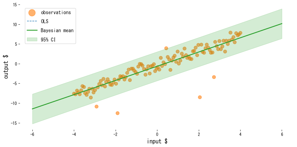
from __future__ import annotations

import japanize_matplotlib
import matplotlib.pyplot as plt
import numpy as np
from sklearn.linear_model import BayesianRidge, LinearRegression
from sklearn.metrics import mean_squared_error


def run_bayesian_linear_demo(
    n_samples: int = 120,
    noise_scale: float = 1.0,
    outlier_count: int = 6,
    outlier_scale: float = 8.0,
    label_observations: str = "observations",
    label_ols: str = "OLS",
    label_bayes: str = "Bayesian mean",
    label_interval: str = "95% CI",
    xlabel: str = "input $",
    ylabel: str = "output $",
    title: str | None = None,
) -> dict[str, float]:
    """Fit OLS and Bayesian ridge to noisy data with outliers, plotting results.

    Args:
        n_samples: Number of evenly spaced sample points.
        noise_scale: Standard deviation of Gaussian noise added to the base line.
        outlier_count: Number of indices to perturb strongly.
        outlier_scale: Standard deviation for the outlier noise.
        label_observations: Legend label for observations.
        label_ols: Label for the ordinary least squares line.
        label_bayes: Label for the Bayesian posterior mean line.
        label_interval: Label for the confidence interval band.
        xlabel: X-axis label.
        ylabel: Y-axis label.
        title: Optional plot title.

    Returns:
        Dictionary containing MSEs and coefficients statistics.
    """
    japanize_matplotlib.japanize()
    rng = np.random.default_rng(seed=0)

    x_values: np.ndarray = np.linspace(-4.0, 4.0, n_samples, dtype=float)
    y_clean: np.ndarray = 1.8 * x_values - 0.5
    y_noisy: np.ndarray = y_clean + rng.normal(scale=noise_scale, size=x_values.shape)

    outlier_idx = rng.choice(n_samples, size=outlier_count, replace=False)
    y_noisy[outlier_idx] += rng.normal(scale=outlier_scale, size=outlier_idx.shape)

    X: np.ndarray = x_values[:, np.newaxis]

    ols = LinearRegression()
    ols.fit(X, y_noisy)
    bayes = BayesianRidge(compute_score=True)
    bayes.fit(X, y_noisy)

    X_grid: np.ndarray = np.linspace(-6.0, 6.0, 200, dtype=float)[:, np.newaxis]
    ols_mean: np.ndarray = ols.predict(X_grid)
    bayes_mean, bayes_std = bayes.predict(X_grid, return_std=True)

    metrics = {
        "ols_mse": float(mean_squared_error(y_noisy, ols.predict(X))),
        "bayes_mse": float(mean_squared_error(y_noisy, bayes.predict(X))),
        "coef_mean": float(bayes.coef_[0]),
        "coef_std": float(np.sqrt(bayes.sigma_[0, 0])),
    }

    upper = bayes_mean + 1.96 * bayes_std
    lower = bayes_mean - 1.96 * bayes_std

    fig, ax = plt.subplots(figsize=(10, 5))
    ax.scatter(X, y_noisy, color="#ff7f0e", alpha=0.6, label=label_observations)
    ax.plot(X_grid, ols_mean, color="#1f77b4", linestyle="--", label=label_ols)
    ax.plot(X_grid, bayes_mean, color="#2ca02c", linewidth=2, label=label_bayes)
    ax.fill_between(
        X_grid.ravel(),
        lower,
        upper,
        color="#2ca02c",
        alpha=0.2,
        label=label_interval,
    )
    ax.set_xlabel(xlabel)
    ax.set_ylabel(ylabel)
    if title:
        ax.set_title(title)
    ax.legend()
    fig.tight_layout()
    plt.show()

    return metrics



metrics = run_bayesian_linear_demo()
print(f"OLS MSE: {metrics['ols_mse']:.3f}")
print(f"Bayesian regression MSE: {metrics['bayes_mse']:.3f}")
print(f"Posterior mean of coefficients: {metrics['coef_mean']:.3f}")
print(f"Posterior std of coefficient: {metrics['coef_std']:.3f}")

bayesian-linear-regression block 1

Reading the results #

OLS is pulled toward the outliers, while Bayesian linear regression keeps the mean prediction more stable.
Using return_std=True yields the predictive standard deviation, which makes it easy to plot credible intervals.
Inspecting the posterior variance highlights which coefficients carry the most uncertainty.

References #

Bishop, C. M. (2006). Pattern Recognition and Machine Learning. Springer.
Murphy, K. P. (2012). Machine Learning: A Probabilistic Perspective. MIT Press.