Linear Regression

Last updated 2020-01-29 Read time 3 min

Summary

Linear regression models the linear relationship between inputs and outputs and provides a baseline that is both predictive and interpretable.
Ordinary least squares estimates the coefficients by minimizing the sum of squared residuals, yielding a closed-form solution.
The slope tells us how much the output changes when the input increases by one unit, while the intercept represents the expected value when the input is zero.
When noise or outliers are large, consider standardization and robust variants so that preprocessing and evaluation remain reliable.

Intuition #

This method should be interpreted through its assumptions, data conditions, and how parameter choices affect generalization.

Detailed Explanation #

Mathematical formulation #

A univariate linear model is written as

$$ y = w x + b. $$

By minimizing the sum of squared residuals $\epsilon_i = y_i - (w x_i + b)$

$$ L(w, b) = \sum_{i=1}^{n} \big(y_i - (w x_i + b)\big)^2, $$

we obtain the analytic solution

$$ w = \frac{\sum_{i=1}^{n} (x_i - \bar{x})(y_i - \bar{y})}{\sum_{i=1}^{n} (x_i - \bar{x})^2}, \qquad b = \bar{y} - w \bar{x}, $$

where $\bar{x}$ and $\bar{y}$ are the means of $x$ and $y$. The same idea extends to multivariate regression with vectors and matrices.

Experiments with Python #

The following code fits a simple regression line with scikit-learn and plots the result. The code is identical to the Japanese page so figures will match across languages.

 1
 2
 3
 4
 5
 6
 7
 8
 9
10
11
12
13
14
15
16
17
18
19
20
21
22
23
24
25
26
27
28
29
30
31
32
33
34
35
36
from __future__ import annotations

import japanize_matplotlib
import matplotlib.pyplot as plt
import numpy as np
from sklearn.linear_model import LinearRegression
from sklearn.pipeline import make_pipeline
from sklearn.preprocessing import StandardScaler

def plot_simple_linear_regression(n_samples: int = 100) -> None:
    """Plot a fitted linear regression model for synthetic data.

    Args:
        n_samples: Number of synthetic samples to generate.
    """
    japanize_matplotlib.japanize()
    rng = np.random.default_rng(seed=0)

    X: np.ndarray = np.linspace(-5.0, 5.0, n_samples, dtype=float)[:, np.newaxis]
    noise: np.ndarray = rng.normal(scale=2.0, size=n_samples)
    y: np.ndarray = 2.0 * X.ravel() + 1.0 + noise

    model = make_pipeline(StandardScaler(with_mean=False), LinearRegression())
    model.fit(X, y)
    y_pred: np.ndarray = model.predict(X)

    fig, ax = plt.subplots(figsize=(10, 5))
    ax.scatter(X, y, marker="x", label="Observed data", c="orange")
    ax.plot(X, y_pred, label="Regression fit")
    ax.set_xlabel("$x$")
    ax.set_ylabel("$y$")
    ax.legend()
    fig.tight_layout()
    plt.show()

plot_simple_linear_regression()

The code is identical to the Japanese page so figures will m… figure

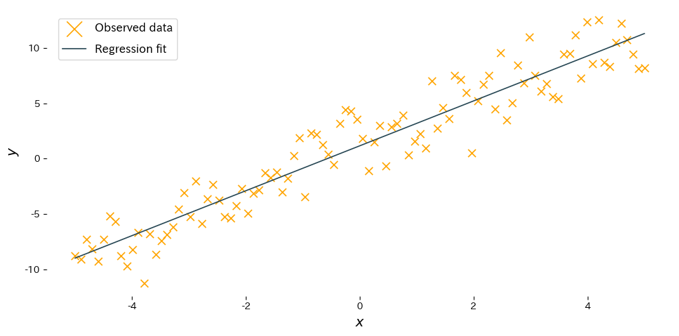
Reading the results #

Slope $w$: indicates how much the output increases or decreases when the input grows by one unit. The estimate should be close to the true slope.
Intercept $b$: shows the expected output when the input is 0, adjusting the vertical position of the line.
Standardizing the features with StandardScaler stabilizes learning when inputs vary in scale.

References #

Draper, N. R., & Smith, H. (1998). Applied Regression Analysis (3rd ed.). John Wiley & Sons.
Hastie, T., Tibshirani, R., & Friedman, J. (2009). The Elements of Statistical Learning. Springer.