Partial Least Squares Regression (PLS)

Last updated 2020-05-20 Read time 3 min

Summary

Partial Least Squares (PLS) extracts latent factors that maximize the covariance between predictors and the target before performing regression.
Unlike PCA, the learned axes incorporate target information, preserving predictive performance while reducing dimensionality.
Tuning the number of latent factors stabilizes models in the presence of strong multicollinearity.
Inspecting loadings reveals which combinations of features are most related to the target.

Intuition #

This method should be interpreted through its assumptions, data conditions, and how parameter choices affect generalization.

Detailed Explanation #

Mathematical formulation #

Given a predictor matrix $\mathbf{X}$ and response vector $\mathbf{y}$, PLS alternates updates of latent scores $\mathbf{t} = \mathbf{X} \mathbf{w}$ and $\mathbf{u} = \mathbf{y} c$ so that their covariance $\mathbf{t}^\top \mathbf{u}$ is maximized. Repeating this procedure yields a set of latent factors on which a linear regression model

$$ \hat{y} = \mathbf{t} \boldsymbol{b} + b_0 $$

is fitted. The number of factors $k$ is typically chosen via cross-validation.

Experiments with Python #

We compare PLS performance for different numbers of latent factors on the Linnerud fitness dataset.

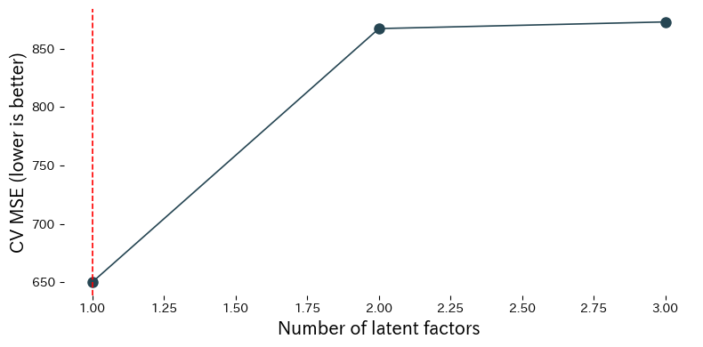
 1
 2
 3
 4
 5
 6
 7
 8
 9
10
11
12
13
14
15
16
17
18
19
20
21
22
23
24
25
26
27
28
29
30
31
32
33
34
35
36
37
38
39
40
41
42
43
44
45
46
47
48
49
50
51
52
53
54
55
56
57
58
59
60
61
62
63
64
65
66
67
68
69
70
71
72
73
74
75
76
77
78
79
80
81
82
83
84
85
86
87
88
89
90
from __future__ import annotations

import japanize_matplotlib
import matplotlib.pyplot as plt
import numpy as np
from sklearn.cross_decomposition import PLSRegression
from sklearn.datasets import load_linnerud
from sklearn.model_selection import KFold, cross_val_score
from sklearn.pipeline import Pipeline
from sklearn.preprocessing import StandardScaler

def evaluate_pls_latent_factors(
    cv_splits: int = 5,
    xlabel: str = "Number of latent factors",
    ylabel: str = "CV MSE (lower is better)",
    label_best: str = "best={k}",
    title: str | None = None,
) -> dict[str, object]:
    """Cross-validate PLS regression for different latent factor counts.

    Args:
        cv_splits: Number of folds for cross-validation.
        xlabel: Label for the number-of-factors axis.
        ylabel: Label for the cross-validation error axis.
        label_best: Format string for the best-factor annotation.
        title: Optional plot title.

    Returns:
        Dictionary with the selected factor count, CV score, and loadings.
    """
    japanize_matplotlib.japanize()
    data = load_linnerud()
    X = data["data"]
    y = data["target"][:, 0]

    max_components = min(X.shape[1], 6)
    components = np.arange(1, max_components + 1)
    cv = KFold(n_splits=cv_splits, shuffle=True, random_state=0)

    scores = []
    pipelines = []
    for k in components:
        model = Pipeline([
            ("scale", StandardScaler()),
            ("pls", PLSRegression(n_components=int(k))),
        ])
        cv_score = cross_val_score(
            model,
            X,
            y,
            cv=cv,
            scoring="neg_mean_squared_error",
        ).mean()
        scores.append(cv_score)
        pipelines.append(model)

    scores_arr = np.array(scores)
    best_idx = int(np.argmax(scores_arr))
    best_k = int(components[best_idx])
    best_mse = float(-scores_arr[best_idx])

    best_model = pipelines[best_idx].fit(X, y)
    x_loadings = best_model["pls"].x_loadings_
    y_loadings = best_model["pls"].y_loadings_

    fig, ax = plt.subplots(figsize=(8, 4))
    ax.plot(components, -scores_arr, marker="o")
    ax.axvline(best_k, color="red", linestyle="--", label=label_best.format(k=best_k))
    ax.set_xlabel(xlabel)
    ax.set_ylabel(ylabel)
    if title:
        ax.set_title(title)
    ax.legend()
    fig.tight_layout()
    plt.show()

    return {
        "best_k": best_k,
        "best_mse": best_mse,
        "x_loadings": x_loadings,
        "y_loadings": y_loadings,
    }

metrics = evaluate_pls_latent_factors()
print(f"Best number of latent factors: {metrics['best_k']}")
print(f"Best CV MSE: {metrics['best_mse']:.3f}")
print("X loadings:
", metrics['x_loadings'])
print("Y loadings:
", metrics['y_loadings'])

We compare PLS performance for different numbers of latent f… figure

Reading the results #

Cross-validated MSE decreases as factors are added, reaches a minimum, and then worsens if you keep adding more.
Inspecting x_loadings_ and y_loadings_ shows which features contribute most to each latent factor.
Standardizing inputs ensures features measured on different scales contribute evenly.

References #

Wold, H. (1975). Soft Modelling by Latent Variables: The Non-Linear Iterative Partial Least Squares (NIPALS) Approach. In Perspectives in Probability and Statistics. Academic Press.
Geladi, P., & Kowalski, B. R. (1986). Partial Least-Squares Regression: A Tutorial. Analytica Chimica Acta, 185, 1–17.