Polynomial Regression

まとめ

Polynomial regression expands features with powers so that a linear model can fit nonlinear relationships.
The model remains a linear combination of coefficients, preserving closed-form solutions and interpretability.
Higher degrees increase expressiveness but also invite overfitting, making regularization and cross-validation important.
Standardizing features and tuning the degree plus penalty strength leads to stable predictions.

Intuition #

A straight line cannot describe smooth curves or hill-shaped patterns. By expanding the input with polynomial terms—$x, x^2, x^3, \dots$ for univariate regression, or powers and interaction terms for multivariate regression—we can express nonlinear behaviour while still using a linear model.

Mathematical formulation #

Given $\mathbf{x} = (x_1, \dots, x_m)$, we build a polynomial feature vector $\phi(\mathbf{x})$ up to degree $d$ and fit a linear regression on top of it. For $m = 2$ and $d = 2$,

$$ \phi(\mathbf{x}) = (1, x_1, x_2, x_1^2, x_1 x_2, x_2^2), $$

and the model becomes

$$ y = \mathbf{w}^\top \phi(\mathbf{x}). $$

As $d$ grows, the number of terms increases rapidly, so in practice we start with degree 2 or 3 and pair it with regularization (e.g., Ridge) when necessary.

Experiments with Python #

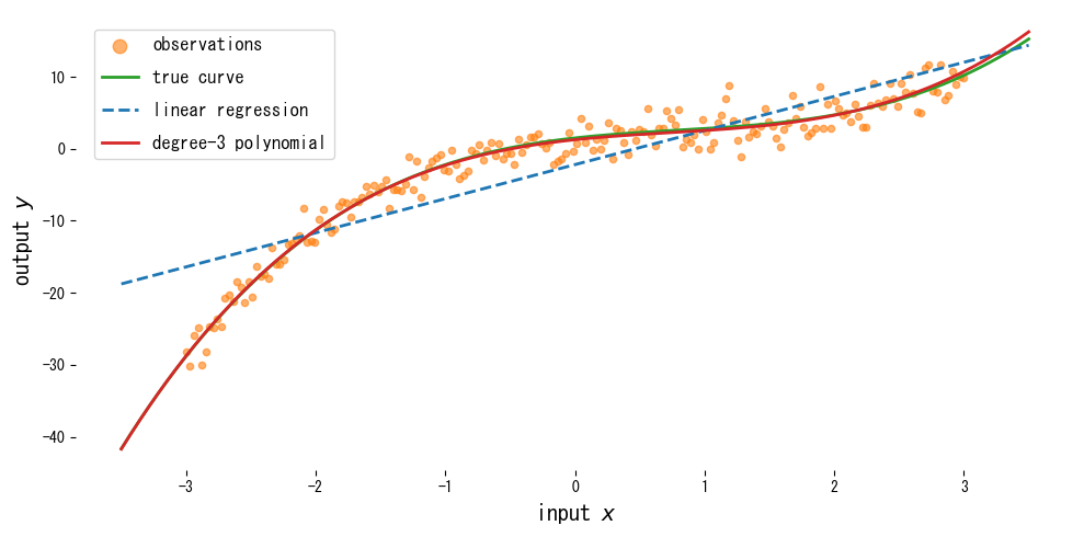
Below we add third-degree polynomial features and fit a curve to data generated from a cubic function plus noise.

from __future__ import annotations

import japanize_matplotlib
import matplotlib.pyplot as plt
import numpy as np
from sklearn.linear_model import LinearRegression
from sklearn.metrics import mean_squared_error
from sklearn.pipeline import make_pipeline
from sklearn.preprocessing import PolynomialFeatures


def compare_polynomial_regression(
    n_samples: int = 200,
    degree: int = 3,
    noise_scale: float = 2.0,
    label_observations: str = "observations",
    label_true_curve: str = "true curve",
    label_linear: str = "linear regression",
    label_poly_template: str = "degree-{degree} polynomial",
) -> tuple[float, float]:
    """Fit linear vs. polynomial regression to a cubic trend and plot the results.

    Args:
        n_samples: Number of synthetic samples generated along the curve.
        degree: Polynomial degree used in the feature expansion.
        noise_scale: Standard deviation of the Gaussian noise added to targets.

    Returns:
        A tuple containing the mean-squared errors of (linear, polynomial) models.
    """
    japanize_matplotlib.japanize()
    rng = np.random.default_rng(seed=42)

    x: np.ndarray = np.linspace(-3.0, 3.0, n_samples, dtype=float)
    y_true: np.ndarray = 0.5 * x**3 - 1.2 * x**2 + 2.0 * x + 1.5
    y_noisy: np.ndarray = y_true + rng.normal(scale=noise_scale, size=x.shape)

    X: np.ndarray = x[:, np.newaxis]

    linear_model = LinearRegression()
    linear_model.fit(X, y_noisy)
    poly_model = make_pipeline(
        PolynomialFeatures(degree=degree, include_bias=False),
        LinearRegression(),
    )
    poly_model.fit(X, y_noisy)

    grid: np.ndarray = np.linspace(-3.5, 3.5, 300, dtype=float)[:, np.newaxis]
    linear_pred: np.ndarray = linear_model.predict(grid)
    poly_pred: np.ndarray = poly_model.predict(grid)
    true_curve: np.ndarray = (
        0.5 * grid.ravel()**3 - 1.2 * grid.ravel()**2 + 2.0 * grid.ravel() + 1.5
    )

    linear_mse: float = float(mean_squared_error(y_noisy, linear_model.predict(X)))
    poly_mse: float = float(mean_squared_error(y_noisy, poly_model.predict(X)))

    fig, ax = plt.subplots(figsize=(10, 5))
    ax.scatter(
        X,
        y_noisy,
        s=20,
        color="#ff7f0e",
        alpha=0.6,
        label=label_observations,
    )
    ax.plot(
        grid,
        true_curve,
        color="#2ca02c",
        linewidth=2,
        label=label_true_curve,
    )
    ax.plot(
        grid,
        linear_pred,
        color="#1f77b4",
        linestyle="--",
        linewidth=2,
        label=label_linear,
    )
    ax.plot(
        grid,
        poly_pred,
        color="#d62728",
        linewidth=2,
        label=label_poly_template.format(degree=degree),
    )
    ax.set_xlabel("input $x$")
    ax.set_ylabel("output $y$")
    ax.legend()
    fig.tight_layout()
    plt.show()

    return linear_mse, poly_mse


degree = 3
linear_mse, poly_mse = compare_polynomial_regression(degree=degree)
print(f"Linear regression MSE: {linear_mse:.3f}")
print(f"Degree-{degree} polynomial regression MSE: {poly_mse:.3f}")

polynomial-regression block 1

Reading the results #

Plain linear regression misses the curvature, especially near the center, while the cubic polynomial follows the true curve closely.
Increasing the degree improves training fit but can make extrapolation unstable.
Combining polynomial features with a regularized regression (e.g., Ridge) via a pipeline helps curb overfitting.

References #

Bishop, C. M. (2006). Pattern Recognition and Machine Learning. Springer.
Hastie, T., Tibshirani, R., & Friedman, J. (2009). The Elements of Statistical Learning. Springer.