Principal Component Regression (PCR)

まとめ

Principal Component Regression (PCR) applies PCA to compress features before fitting linear regression, reducing instability from multicollinearity.
Principal components prioritize directions with large variance, filtering noisy axes while preserving informative structure.
Choosing how many components to keep balances overfitting risk and computational cost.
Proper preprocessing—standardization and handling missing values—lays the groundwork for accuracy and interpretability.

Intuition #

When predictors are highly correlated, least squares can yield wildly varying coefficients. PCR first performs PCA to combine correlated directions, then regresses on the leading principal components ordered by explained variance. By focusing on dominant variation, the resulting coefficients become more stable.

Mathematical formulation #

Apply PCA to the standardized design matrix $\mathbf{X}$ and retain the top $k$ eigenvectors. With principal component scores $\mathbf{Z} = \mathbf{X} \mathbf{W}_k$, the regression model

$$ y = \boldsymbol{\gamma}^\top \mathbf{Z} + b $$

is learned. Coefficients in the original feature space are recovered via $\boldsymbol{\beta} = \mathbf{W}_k \boldsymbol{\gamma}$. The number of components $k$ is selected using cumulative explained variance or cross-validation.

Experiments with Python #

We evaluate cross-validation scores of PCR on the diabetes dataset as we vary the number of components.

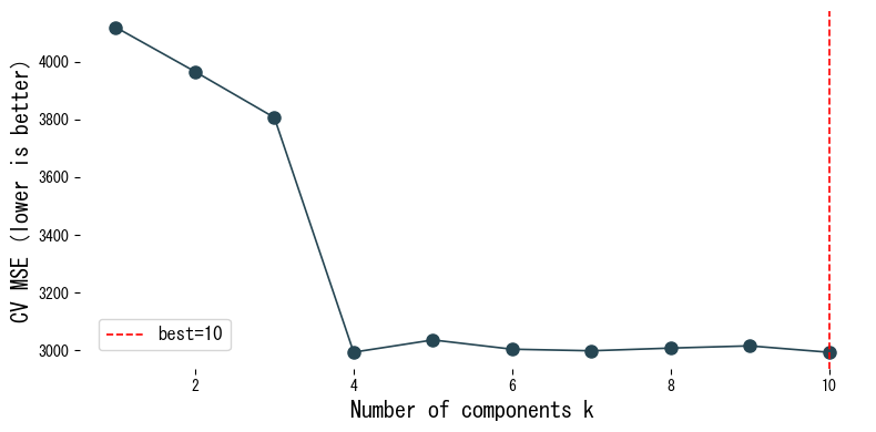
from __future__ import annotations

import japanize_matplotlib
import matplotlib.pyplot as plt
import numpy as np
from sklearn.datasets import load_diabetes
from sklearn.decomposition import PCA
from sklearn.linear_model import LinearRegression
from sklearn.model_selection import cross_val_score
from sklearn.pipeline import Pipeline
from sklearn.preprocessing import StandardScaler


def evaluate_pcr_components(
    cv_folds: int = 5,
    xlabel: str = "Number of components k",
    ylabel: str = "CV MSE (lower is better)",
    title: str | None = None,
    label_best: str = "best={k}",
) -> dict[str, float]:
    """Cross-validate PCR with varying component counts and plot the curve.

    Args:
        cv_folds: Number of folds for cross-validation.
        xlabel: Label for the component-count axis.
        ylabel: Label for the error axis.
        title: Optional title for the plot.
        label_best: Format string for highlighting the best component count.

    Returns:
        Dictionary containing the best component count and its CV score.
    """
    japanize_matplotlib.japanize()
    X, y = load_diabetes(return_X_y=True)

    def build_pcr(n_components: int) -> Pipeline:
        return Pipeline([
            ("scale", StandardScaler()),
            ("pca", PCA(n_components=n_components, random_state=0)),
            ("reg", LinearRegression()),
        ])

    components = np.arange(1, X.shape[1] + 1)
    cv_scores = []
    for k in components:
        model = build_pcr(int(k))
        score = cross_val_score(
            model,
            X,
            y,
            cv=cv_folds,
            scoring="neg_mean_squared_error",
        )
        cv_scores.append(score.mean())

    cv_scores_arr = np.array(cv_scores)
    best_idx = int(np.argmax(cv_scores_arr))
    best_k = int(components[best_idx])
    best_mse = float(-cv_scores_arr[best_idx])

    best_model = build_pcr(best_k).fit(X, y)
    explained = best_model["pca"].explained_variance_ratio_

    fig, ax = plt.subplots(figsize=(8, 4))
    ax.plot(components, -cv_scores_arr, marker="o")
    ax.axvline(best_k, color="red", linestyle="--", label=label_best.format(k=best_k))
    ax.set_xlabel(xlabel)
    ax.set_ylabel(ylabel)
    if title:
        ax.set_title(title)
    ax.legend()
    fig.tight_layout()
    plt.show()

    return {
        "best_k": best_k,
        "best_mse": best_mse,
        "explained_variance_ratio": explained,
    }



metrics = evaluate_pcr_components()
print(f"Best number of components: {metrics['best_k']}")
print(f"Best CV MSE: {metrics['best_mse']:.3f}")
print("Explained variance ratio:", metrics['explained_variance_ratio'])

principal-component-regression block 1

Reading the results #

As the number of components increases, the training fit improves, but cross-validated MSE reaches a minimum at an intermediate value.
Inspecting the explained variance ratio reveals how much of the overall variability each component captures.
Component loadings indicate which original features contribute most to each principal direction.

References #

Jolliffe, I. T. (2002). Principal Component Analysis (2nd ed.). Springer.
Massy, W. F. (1965). Principal Components Regression in Exploratory Statistical Research. Journal of the American Statistical Association, 60(309), 234–256.