Weighted Least Squares (WLS)

まとめ

Weighted least squares assigns observation-specific weights so trustworthy measurements influence the fitted line more strongly.
Multiplying squared errors by weights downplays high-variance observations and keeps the estimate close to reliable data.
You can run WLS with scikit-learn’s LinearRegression by providing sample_weight.
Weights can stem from known variances, residual diagnostics, or domain knowledge; careful design is crucial.

Intuition #

Ordinary least squares assumes every observation is equally reliable, yet real-world sensors often vary in precision. WLS “listens” more to the data points you trust by emphasizing them during fitting, allowing the familiar linear regression framework to handle heteroscedastic data.

Mathematical formulation #

With positive weights $w_i$, minimize

$$ L(\boldsymbol\beta, b) = \sum_{i=1}^{n} w_i \left(y_i - (\boldsymbol\beta^\top \mathbf{x}_i + b)\right)^2. $$

The optimal choice $w_i \propto 1/\sigma_i^2$ (inverse variance) gives more influence to precise observations.

Experiments with Python #

We compare OLS and WLS on data whose noise level differs across regions.

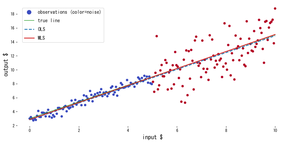
from __future__ import annotations

import japanize_matplotlib
import matplotlib.pyplot as plt
import numpy as np
from sklearn.linear_model import LinearRegression


def run_weighted_vs_ols(
    n_samples: int = 200,
    threshold: float = 5.0,
    low_noise: float = 0.5,
    high_noise: float = 2.5,
    xlabel: str = "input $",
    ylabel: str = "output $",
    label_scatter: str = "observations (color=noise)",
    label_truth: str = "true line",
    label_ols: str = "OLS",
    label_wls: str = "WLS",
    title: str | None = None,
) -> dict[str, float]:
    """Compare OLS and weighted least squares on heteroscedastic data.

    Args:
        n_samples: Number of evenly spaced samples to generate.
        threshold: Breakpoint separating low- and high-noise regions.
        low_noise: Noise scale for the lower region.
        high_noise: Noise scale for the higher region.
        xlabel: Label for the x-axis.
        ylabel: Label for the y-axis.
        label_scatter: Legend label for the colored scatter plot.
        label_truth: Legend label for the ground-truth line.
        label_ols: Legend label for the OLS fit.
        label_wls: Legend label for the WLS fit.
        title: Optional title for the plot.

    Returns:
        Dictionary with slopes and intercepts of both fits.
    """
    japanize_matplotlib.japanize()
    rng = np.random.default_rng(7)

    X_vals: np.ndarray = np.linspace(0.0, 10.0, n_samples, dtype=float)
    true_y: np.ndarray = 1.2 * X_vals + 3.0

    noise_scale = np.where(X_vals < threshold, low_noise, high_noise)
    y_noisy = true_y + rng.normal(scale=noise_scale)

    weights = 1.0 / (noise_scale**2)
    X = X_vals[:, np.newaxis]

    ols = LinearRegression()
    ols.fit(X, y_noisy)

    wls = LinearRegression()
    wls.fit(X, y_noisy, sample_weight=weights)

    grid = np.linspace(0.0, 10.0, 200, dtype=float)[:, np.newaxis]
    ols_pred = ols.predict(grid)
    wls_pred = wls.predict(grid)

    fig, ax = plt.subplots(figsize=(10, 5))
    scatter = ax.scatter(
        X,
        y_noisy,
        c=noise_scale,
        cmap="coolwarm",
        s=25,
        label=label_scatter,
    )
    ax.plot(grid, 1.2 * grid.ravel() + 3.0, color="#2ca02c", label=label_truth)
    ax.plot(grid, ols_pred, color="#1f77b4", linestyle="--", linewidth=2, label=label_ols)
    ax.plot(grid, wls_pred, color="#d62728", linewidth=2, label=label_wls)
    ax.set_xlabel(xlabel)
    ax.set_ylabel(ylabel)
    if title:
        ax.set_title(title)
    ax.legend()
    fig.tight_layout()
    plt.show()

    return {
        "ols_slope": float(ols.coef_[0]),
        "ols_intercept": float(ols.intercept_),
        "wls_slope": float(wls.coef_[0]),
        "wls_intercept": float(wls.intercept_),
    }



metrics = run_weighted_vs_ols()
print(f"OLS slope: {metrics['ols_slope']:.3f}, intercept: {metrics['ols_intercept']:.3f}")
print(f"WLS slope: {metrics['wls_slope']:.3f}, intercept: {metrics['wls_intercept']:.3f}")

weighted-least-squares block 1

Reading the results #

Weighting draws the fit toward the low-noise region, producing estimates close to the true line.
OLS is skewed by the noisy region and underestimates the slope.
Performance hinges on choosing appropriate weights; diagnostics and domain intuition matter.

References #

Carroll, R. J., & Ruppert, D. (1988). Transformation and Weighting in Regression. Chapman & Hall.
Seber, G. A. F., & Lee, A. J. (2012). Linear Regression Analysis (2nd ed.). Wiley.