2.3.1
Decision Tree (Classifier)
- A decision tree classifier partitions the feature space with a sequence of if-then questions so that each terminal node contains mostly one class.
- Split quality is measured with impurity scores such as the Gini index or entropy; choose the score that best reflects the cost of misclassification for your task.
- Controlling depth, minimum samples per node, or pruning keeps the tree from memorising noise while preserving interpretability.
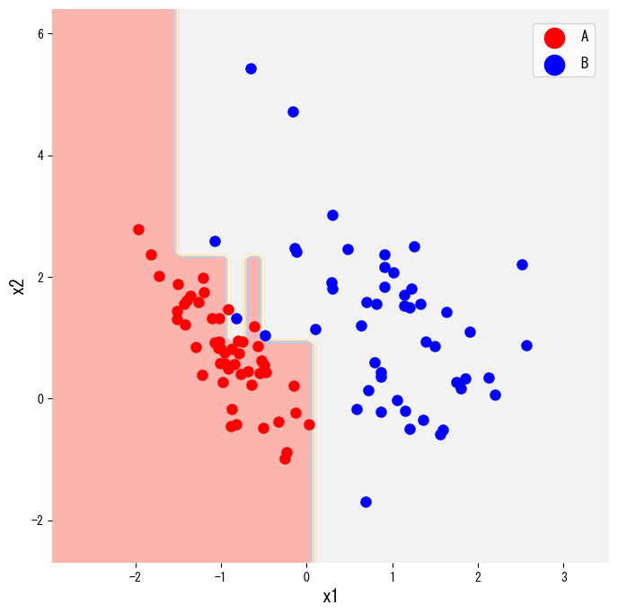
- Visualising both the decision regions and the learned tree helps explain the model to stakeholders.
Intuition #
This method should be interpreted through its assumptions, data conditions, and how parameter choices affect generalization.
Detailed Explanation #
1. Overview #
Decision trees are supervised learning models that recursively split the input space. Starting from the root, each internal node asks a question like “is (x_j \le s)?” and routes the sample to the next node. For classification we want leaves that are as pure as possible, meaning they contain almost only one class label. The final model is therefore a compact rule book that can easily be inspected or converted into business logic.
2. Impurity measures #
Let (t) be a node and (p_k) the class proportion inside that node. Two common impurity scores are
$$ \mathrm{Gini}(t) = 1 - \sum_k p_k^2, $$$$ H(t) = - \sum_k p_k \log p_k. $$When splitting node (t) on feature (x_j) with threshold (s), we evaluate the gain
$$ \Delta I = I(t) - \frac{n_L}{n_t} I(t_L) - \frac{n_R}{n_t} I(t_R), $$where (I(\cdot)) is either Gini or entropy, (t_L) and (t_R) are the child nodes, and (n_t) is the number of samples reaching (t). The split that maximises (\Delta I) is selected.
3. Python example #
The snippet below generates a two-class toy dataset with make_classification, fits a DecisionTreeClassifier, and visualises its decision regions. Changing criterion from "gini" to "entropy" switches the impurity measure.
| |
The same estimator can be rendered as an actual tree diagram with plot_tree, which is convenient for reports or slide decks.
| |

4. References #
- Breiman, L., Friedman, J. H., Olshen, R. A., & Stone, C. J. (1984). Classification and Regression Trees. Wadsworth.
- scikit-learn developers. (2024). Decision Trees. https://scikit-learn.org/stable/modules/tree.html