2.3.2
Decision Tree (Regressor)
- Regression trees approximate nonlinear relationships by recursively splitting the feature space until each leaf can be represented by a single constant value.
- Splits minimise the mean squared error (MSE) of the left and right children; the reduction in MSE determines whether a question is useful.
- Hyperparameters such as
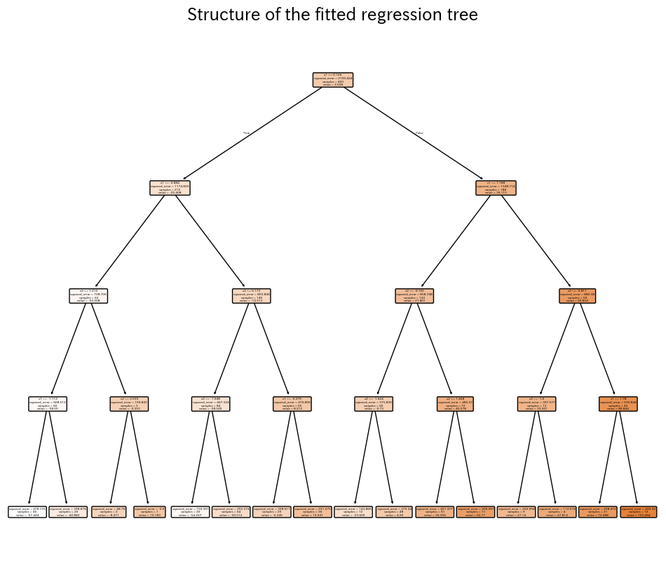
max_depth,min_samples_leaf, andccp_alphabalance accuracy against interpretability and help avoid overfitting. - Visual diagnostics—scatter plots, contour maps, and rendered trees—make it easy to explain which regions share the same prediction.
- Decision Tree Classifier — understanding this concept first will make learning smoother
Intuition #
This method should be interpreted through its assumptions, data conditions, and how parameter choices affect generalization.
Detailed Explanation #
1. Overview #
Like classifiers, regression trees ask simple questions about the input features, but the target is continuous. Each leaf predicts a constant (the average of training samples that arrived there). Because the function is piecewise constant, increasing depth captures increasingly fine-grained structure, while shallow trees emphasise smooth trends.
2. Split criterion (variance reduction) #
For a node (t) containing (n_t) samples and average target (\bar{y}_t), the impurity is the node MSE:
$$ \mathrm{MSE}(t) = \frac{1}{n_t} \sum_{i \in t} (y_i - \bar{y}_t)^2. $$Splitting on (x_j) at threshold (s) yields children (t_L) and (t_R). The quality of the split is measured by
$$ \Delta = \mathrm{MSE}(t) - \frac{n_L}{n_t} \mathrm{MSE}(t_L) - \frac{n_R}{n_t} \mathrm{MSE}(t_R). $$We choose the split with the largest (\Delta); when no split yields positive gain, the node becomes a leaf.
3. Python example #
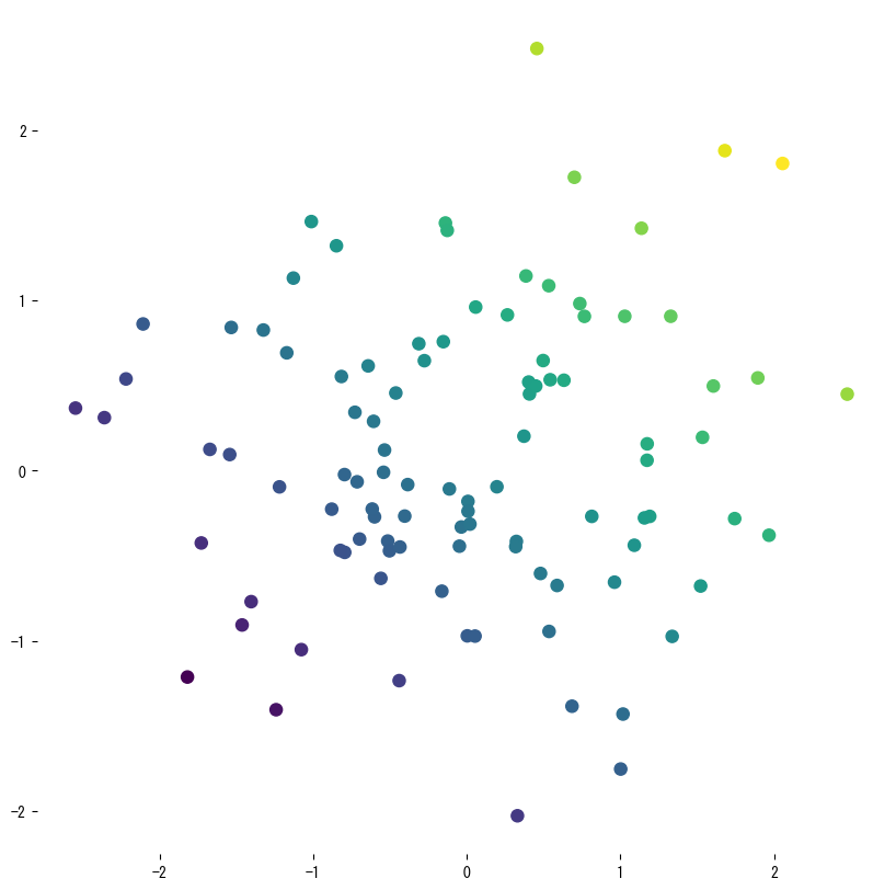
The first snippet fits a shallow tree to noisy samples drawn from a sine curve so we can see the piecewise-constant nature of the prediction. A second experiment trains a two-feature regressor, evaluates (R^2), RMSE, and MAE, and visualises the learned surface plus the final tree.
| |
| |
| |

4. References #
- Breiman, L., Friedman, J. H., Olshen, R. A., & Stone, C. J. (1984). Classification and Regression Trees. Wadsworth.
- scikit-learn developers. (2024). Decision Trees. https://scikit-learn.org/stable/modules/tree.html