Decision Tree Parameters | Tuning depth, leaves, and pruning

1. Overview #

A decision tree grows by repeatedly picking the split that yields the largest impurity decrease. Without constraints the tree keeps splitting until every leaf is pure, which often means overfitting. Hyperparameters therefore act as regularisers: depth limits keep the tree shallow, minimum sample counts avoid tiny leaves, and pruning collapses branches whose contribution is marginal.

2. Impurity gain and cost-complexity pruning #

For a parent node (P) split into children (L) and (R), the impurity decrease is

$$ \Delta I = I(P) - \frac{|L|}{|P|} I(L) - \frac{|R|}{|P|} I(R), $$

where (I(\cdot)) can be the Gini index, entropy, MSE, or MAE depending on the task. A split is only kept if (\Delta I > 0).

Cost-complexity pruning scores an entire tree (T) with

$$ R_\alpha(T) = R(T) + \alpha |T|, $$

where (R(T)) is the training loss (e.g., total squared error), (|T|) is the number of leaves, and (\alpha \ge 0) penalises large trees. Increasing (\alpha) encourages simpler structures.

3. Python experiments #

The snippet below trains several DecisionTreeRegressor models on a synthetic dataset and reports how different hyperparameters affect the training and validation (R^2). Adjusting max_depth, min_samples_leaf, or ccp_alpha shows how capacity and generalisation trade off.

import numpy as np
import matplotlib.pyplot as plt
from sklearn.model_selection import train_test_split
from sklearn.tree import DecisionTreeRegressor
from sklearn.datasets import make_regression
from sklearn.metrics import r2_score

X, y = make_regression(
    n_samples=500,
    n_features=2,
    noise=0.2,
    random_state=42,
)
Xtr, Xte, ytr, yte = train_test_split(X, y, test_size=0.3, random_state=0)

def evaluate(params):
    model = DecisionTreeRegressor(random_state=0, **params).fit(Xtr, ytr)
    r2_train = r2_score(ytr, model.predict(Xtr))
    r2_test = r2_score(yte, model.predict(Xte))
    print(f"{params}: train R2={r2_train:.3f}, test R2={r2_test:.3f}")

evaluate({"max_depth": 3})
evaluate({"max_depth": 10})
evaluate({"max_depth": 5, "min_samples_leaf": 5})
evaluate({"max_depth": 5, "ccp_alpha": 0.01})

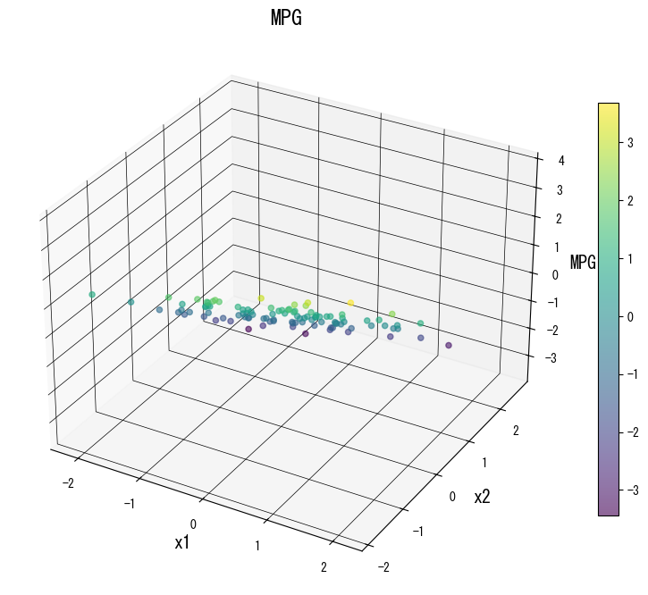
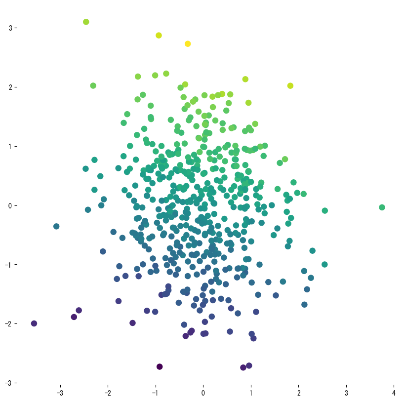
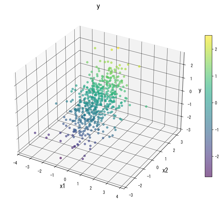
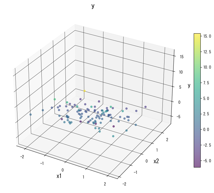
The following figures (shared with the Japanese page) illustrate how varying key knobs reshapes the prediction surface. Use them as a visual checklist when tuning your own tree:

4. References #