4.3.0
Confusion Matrix
- Understand the fundamentals of this metric, what it evaluates, and how to interpret the results.
- Compute and visualise the metric with Python 3.13 code examples, covering key steps and practical checkpoints.
- Combine charts and complementary metrics for effective model comparison and threshold tuning.
1. Anatomy of a confusion matrix #
For binary classification the matrix is a 2×2 table:
| Predicted: Negative | Predicted: Positive | |
|---|---|---|
| Actual: Negative | True Negative (TN) | False Positive (FP) |
| Actual: Positive | False Negative (FN) | True Positive (TP) |
- Rows represent the ground truth, columns the model prediction.
- Inspecting TP / FP / FN / TN reveals whether the model is biased toward a specific class.
2. End-to-end example on Python 3.13 #
Make sure you are running Python 3.13 and install the required libraries:
| |
The script below trains a logistic regression model on the breast cancer dataset, then prints and plots the confusion matrix. A Pipeline with StandardScaler keeps the optimisation stable and avoids convergence warnings.
| |
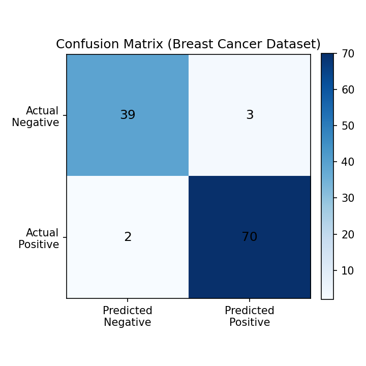
Confusion matrix rendered with scikit-learn (Python 3.13)
3. Normalising the matrix #
When the dataset is imbalanced, normalising by row (actual labels) helps you compare error rates.
| |
normalize="true": ratio within each actual classnormalize="pred": ratio within each predicted classnormalize="all": ratio over all observations
4. Extending to multiclass problems #
ConfusionMatrixDisplay.from_predictions automatically builds the matrix for multiclass tasks and adds axis labels.
| |
5. Practical checkpoints #
- False negatives vs. false positives: decide which error is more costly (e.g., medical diagnosis vs. fraud detection) and monitor the relevant cells closely.
- Pair with heatmaps: visual inspection highlights skewed classes and makes cross-team discussions easier.
- Derive other metrics: accuracy, precision, recall, and F1 can all be computed from the same matrix. Compare them with ROC-AUC or PR curves for a fuller picture.
- Keep notebooks reproducible: packaging the analysis in a Python 3.13 notebook enables fast iteration when you tune or retrain the model.
Summary #
A confusion matrix summarises TP / FP / FN / TN and exposes the bias of a classifier.
Normalising the matrix reveals error ratios when classes are imbalanced.
Combine the matrix with derived metrics and business requirements to define actionable evaluation criteria.