Log Loss

Last updated 2020-03-11 Read time 2 min

Summary

Understand the fundamentals of this metric, what it evaluates, and how to interpret the results.
Compute and visualise the metric with Python 3.13 code examples, covering key steps and practical checkpoints.
Combine charts and complementary metrics for effective model comparison and threshold tuning.

1. Definition #

For binary classification the loss is \mathrm{LogLoss} = -\frac{1}{n} \sum_{i=1}^{n} \bigl[y_i \log(p_i) + (1 - y_i) \log(1 - p_i)\bigr], where \(p_i\) is the predicted probability of the positive class and \(y_i \in {0,1}\) is the true label. Multiclass log loss extends this by summing over classes with one-hot targets.

2. Computing with Python 3.13 #

1
2
python --version        # e.g. Python 3.13.0
pip install scikit-learn matplotlib

 1
 2
 3
 4
 5
 6
 7
 8
 9
10
11
12
13
14
15
16
17
18
from sklearn.datasets import load_breast_cancer
from sklearn.linear_model import LogisticRegression
from sklearn.metrics import classification_report, log_loss
from sklearn.model_selection import train_test_split
from sklearn.pipeline import make_pipeline
from sklearn.preprocessing import StandardScaler
X, y = load_breast_cancer(return_X_y=True)
X_train, X_test, y_train, y_test = train_test_split(
    X, y, test_size=0.3, stratify=y, random_state=42
)
model = make_pipeline(
    StandardScaler(),
    LogisticRegression(max_iter=2000, solver="lbfgs"),
)
model.fit(X_train, y_train)
proba = model.predict_proba(X_test)
print(classification_report(y_test, model.predict(X_test), digits=3))
print("Log Loss:", log_loss(y_test, proba))

Just pass the probability array from predict_proba into log_loss.

3. Intuition from the penalty curves #

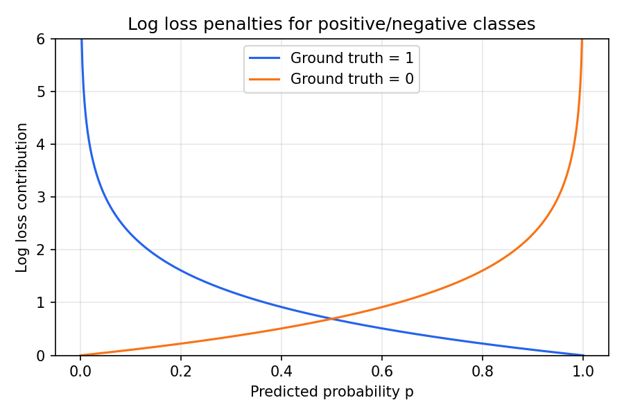
Log loss penalty — Predicted probabilities close to the wrong class trigger a steep penalty.

Giving a low probability to a positive example (e.g. 0.1) yields a large penalty.
Returning 0.5 for every sample (i.e. being unsure) is also penalised—the model makes no useful distinction.

4. Where to use Log Loss #

Calibration checks – after Platt scaling or isotonic regression, verify that Log Loss decreased.
Competitions and leaderboards – Kaggle and similar platforms often use Log Loss to rank probabilistic models.
Threshold-free comparison – unlike Accuracy, Log Loss evaluates the entire distribution of probabilities. The log_loss function exposes options such as labels, eps, and ormalize to handle missing labels and numerical stability.

Summary #

Log Loss measures how far predicted probabilities deviate from reality; lower values are better.
Python 3.13 + scikit-learn make it a one-liner once you have probability outputs.
Pair it with ranking metrics like ROC-AUC or PR curves to assess both discrimination and calibration.