Coefficient of determination

The coefficient of determination is a value in statistics that expresses how much of the dependent variable (objective variable) is explained by the independent variable (explanatory variable).

Generally, the higher the better the rating indicator
The best case is 1.
However, the more features you add, the higher the score tends to be.
Therefore, it is not possible to judge “high accuracy of the model” by looking at this indicator alone

import numpy as np
import matplotlib.pyplot as plt
import japanize_matplotlib
from sklearn.datasets import make_regression
from sklearn.ensemble import RandomForestRegressor
from sklearn.model_selection import train_test_split

Create models and calculate coefficients of determination for sample data #

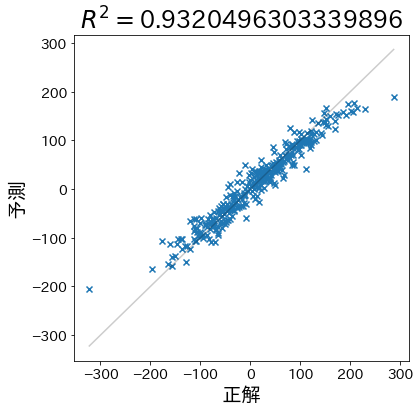
First, let’s create data that makes predictions more likely to be correct.

X, y = make_regression(
    n_samples=1000,
    n_informative=3,
    n_features=20,
    random_state=RND,
)
train_X, test_X, train_y, test_y = train_test_split(
    X, y, test_size=0.33, random_state=RND
)

model = RandomForestRegressor(max_depth=5)
model.fit(train_X, train_y)
pred_y = model.predict(test_X)

Calculate coefficient of determination #

sklearn.metrics.roc_auc_score

from sklearn.metrics import r2_score

r2 = r2_score(test_y, pred_y)
y_min, y_max = np.min(test_y), np.max(test_y)

plt.figure(figsize=(6, 6))
plt.title(f"$R^2 =${r2}")
plt.plot([y_min, y_max], [y_min, y_max], linestyle="-", c="k", alpha=0.2)
plt.scatter(test_y, pred_y, marker="x")
plt.xlabel("target")
plt.ylabel("prediction")

png

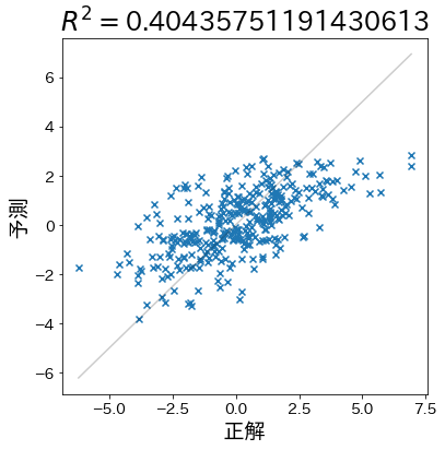
Next, create data for which the predictions are less likely to be correct and check to see that the coefficient of determination falls.

X, y = make_regression(
    n_samples=1000,
    n_informative=3,
    n_features=20,
    effective_rank=4,
    noise=1.5,
    random_state=RND,
)
train_X, test_X, train_y, test_y = train_test_split(
    X, y, test_size=0.33, random_state=RND
)

model = RandomForestRegressor(max_depth=5)
model.fit(train_X, train_y)
pred_y = model.predict(test_X)

r2 = r2_score(test_y, pred_y)
y_min, y_max = np.min(test_y), np.max(test_y)

plt.figure(figsize=(6, 6))
plt.title(f"$R^2 =${r2}")
plt.plot([y_min, y_max], [y_min, y_max], linestyle="-", c="k", alpha=0.2)
plt.scatter(test_y, pred_y, marker="x")
plt.xlabel("target")
plt.ylabel("prediction")

png

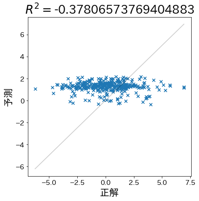
When the prediction is almost random #

When the accuracy is even worse than simply predicting the average, the coefficient of determination is negative.

X, y = make_regression(
    n_samples=1000,
    n_informative=3,
    n_features=20,
    effective_rank=4,
    noise=1.5,
    random_state=RND,
)
train_X, test_X, train_y, test_y = train_test_split(
    X, y, test_size=0.33, random_state=RND
)

# Randomly reorder train_y and convert values
train_y = np.random.permutation(train_y)
train_y = np.sin(train_y) * 10 + 1

model = RandomForestRegressor(max_depth=1)
model.fit(train_X, train_y)
pred_y = model.predict(test_X)

r2 = r2_score(test_y, pred_y)
y_min, y_max = np.min(test_y), np.max(test_y)

plt.figure(figsize=(6, 6))
plt.title(f"$R^2 =${r2}")
plt.plot([y_min, y_max], [y_min, y_max], linestyle="-", c="k", alpha=0.2)
plt.scatter(test_y, pred_y, marker="x")
plt.xlabel("target")
plt.ylabel("prediction")

png

Coefficient of determination when using the least squares method #

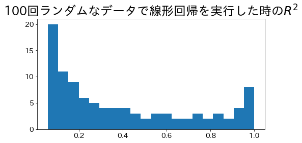
In the case of a regression line for a single regression using the least squares method, the range of the coefficient of determination is $ 0 \le R^2 \le 1$. Let us try to find the coefficient of determination by running a 100-line regression with random noise on the data.

from sklearn.linear_model import LinearRegression
from sklearn.pipeline import make_pipeline
from sklearn.preprocessing import StandardScaler

r2_scores = []
for i in range(100):
    X, y = make_regression(
        n_samples=500,
        n_informative=1,
        n_features=1,
        effective_rank=4,
        noise=i * 0.1,
        random_state=RND,
    )
    train_X, test_X, train_y, test_y = train_test_split(
        X, y, test_size=0.33, random_state=RND
    )

    # linear regression
    model = make_pipeline(
        StandardScaler(with_mean=False), LinearRegression(positive=True)
    ).fit(train_X, train_y)

    # Calculate coefficient of determination
    pred_y = model.predict(test_X)
    r2 = r2_score(test_y, pred_y)
    r2_scores.append(r2)


plt.figure(figsize=(8, 4))
plt.hist(r2_scores, bins=20)
plt.show()

png