mplfinance is an extension to matplotlib for visualising financial data. In this article we create graphs from financial data using mplfinance. The basic usage is explained in the Tutorials section of the mplfinance repository.
Loading Data
#
1
2
3
4
5
| import os
import time
import pandas as pd
import pandas_datareader.data as web
from pandas_datareader._utils import RemoteDataError
|
 1
 2
 3
 4
 5
 6
 7
 8
 9
10
11
12
13
14
15
16
17
18
19
20
21
22
23
24
25
26
27
28
29
30
31
| def get_finance_data(
ticker_symbol: str, start="2021-01-01", end="2021-06-30", savedir="data"
) -> pd.DataFrame:
"""Retrieves data recording stock prices
Args:
ticker_symbol (str): Description of param1
start (str): Date of beginning of period, optional.
end (str): Date of end of period, optional.
Returns:
res: Stock Price Data
"""
res = None
filepath = os.path.join(savedir, f"{ticker_symbol}_{start}_{end}_historical.csv")
os.makedirs(savedir, exist_ok=True)
if not os.path.exists(filepath):
try:
time.sleep(5.0)
res = web.DataReader(ticker_symbol, "yahoo", start=start, end=end)
res.to_csv(filepath, encoding="utf-8-sig")
except (RemoteDataError, KeyError):
print(f"ticker_symbol ${ticker_symbol} が正しいか確認してください。")
else:
res = pd.read_csv(filepath, index_col="Date")
res.index = pd.to_datetime(res.index)
assert res is not None, "データ取得に失敗しました"
return res
|
1
2
3
4
5
6
7
| # ticker symbol, period, and destination file
ticker_symbol = "NVDA"
start = "2021-01-01"
end = "2021-06-30"
df = get_finance_data(ticker_symbol, start=start, end=end, savedir="../data")
df.head()
|
| High | Low | Open | Close | Volume | Adj Close |
|---|
| Date | | | | | | |
|---|
| 2020-12-31 | 131.509995 | 129.149994 | 131.365005 | 130.550003 | 19242400.0 | 130.413864 |
|---|
| 2021-01-04 | 136.524994 | 129.625000 | 131.042496 | 131.134995 | 56064000.0 | 130.998245 |
|---|
| 2021-01-05 | 134.434998 | 130.869995 | 130.997498 | 134.047501 | 32276000.0 | 133.907700 |
|---|
| 2021-01-06 | 132.449997 | 125.860001 | 132.225006 | 126.144997 | 58042400.0 | 126.013443 |
|---|
| 2021-01-07 | 133.777496 | 128.865005 | 129.675003 | 133.440002 | 46148000.0 | 133.300842 |
|---|
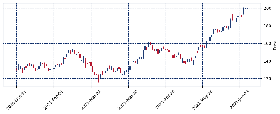
Plotting OHLC
#
OHLC is the opening price, high, low, and close, and is one of the graphs we usually look at most often.
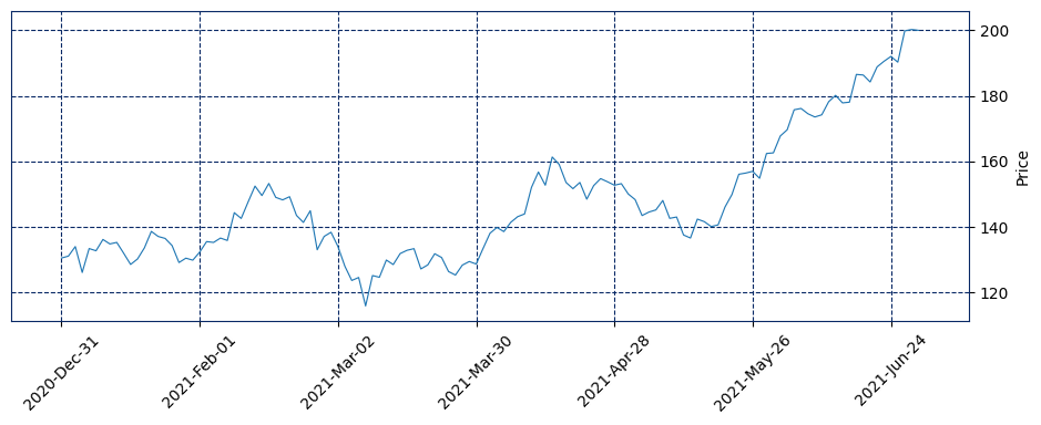
Let’s plot it as a candlestick and as a line.
1
2
3
4
| import mplfinance as mpf
mpf.plot(df, type="candle", style="starsandstripes", figsize=(12, 4))
mpf.plot(df, type="line", style="starsandstripes", figsize=(12, 4))
|
Moving Average
#
One of the indicators used in technical analysis of stock prices and foreign exchange is the moving average.
In current technical analysis, there are many examples where three moving averages (short, medium, and long term) are displayed simultaneously. In daily charts, the 5-day, 25-day, and 75-day moving averages are often used.
Specify the mav option to plot the 5/25/75 day moving average.
1
| mpf.plot(df, type="candle", style="starsandstripes", figsize=(12, 4), mav=[5, 25, 75])
|
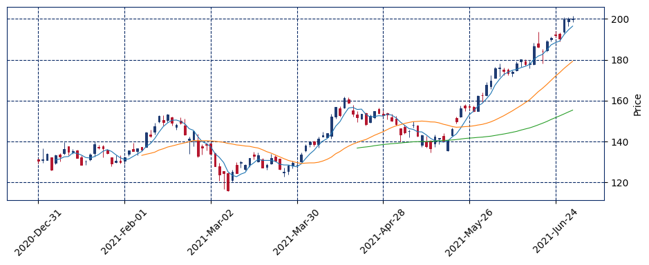
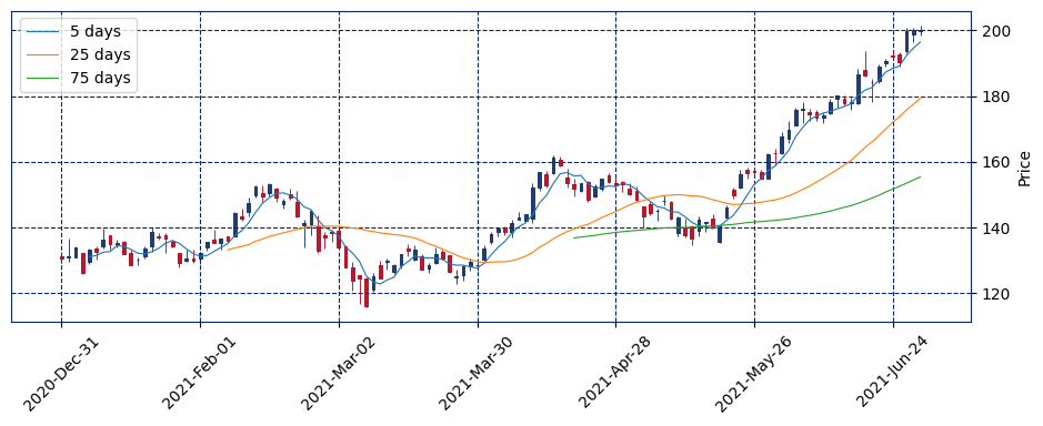
Show legend
#
Add a legend because it is difficult to tell which line represents a moving average over what number of days.
 1
 2
 3
 4
 5
 6
 7
 8
 9
10
11
12
13
14
| import japanize_matplotlib
import matplotlib.patches as mpatches
fig, axes = mpf.plot(
df,
type="candle",
style="starsandstripes",
figsize=(12, 4),
mav=[5, 25, 75],
returnfig=True,
)
fig.legend(
[f"{days} days" for days in [5, 25, 75]], bbox_to_anchor=(0.0, 0.78, 0.28, 0.102)
)
|
<matplotlib.legend.Legend at 0x7f8be96e5b80>
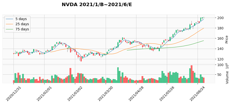
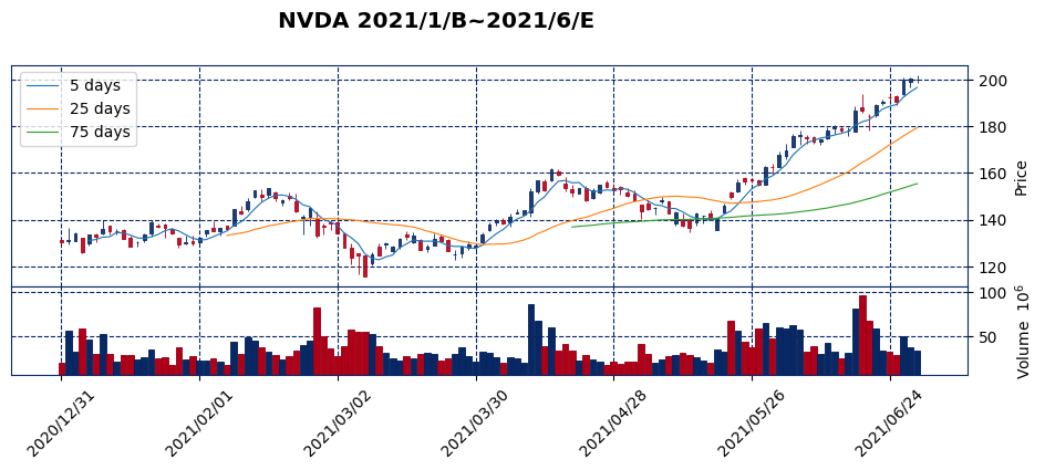
Displaying Volume
#
 1
 2
 3
 4
 5
 6
 7
 8
 9
10
11
12
13
14
| fig, axes = mpf.plot(
df,
title="NVDA 2021/1/B~2021/6/E",
type="candle",
style="starsandstripes",
figsize=(12, 4),
mav=[5, 25, 75],
volume=True,
datetime_format="%Y/%m/%d",
returnfig=True,
)
fig.legend(
[f"{days} days" for days in [5, 25, 75]], bbox_to_anchor=(0.0, 0.78, 0.28, 0.102)
)
|
 1
 2
 3
 4
 5
 6
 7
 8
 9
10
11
12
13
14
| fig, axes = mpf.plot(
df,
title="NVDA 2021/1/B~2021/6/E",
type="candle",
style="yahoo",
figsize=(12, 4),
mav=[5, 25, 75],
volume=True,
datetime_format="%Y/%m/%d",
returnfig=True,
)
fig.legend(
[f"{days} days" for days in [5, 25, 75]], bbox_to_anchor=(0.0, 0.78, 0.28, 0.102)
)
|