3.3.1
Binning numerical features
<p><b>Binning</b> (discretisation) converts a continuous feature into ordered categories. It is useful when a model cannot handle real-valued inputs directly or when you wish to build features such as an “income decile”.</p>
Equal-width vs. equal-frequency #
Let (x_1, \dots, x_n) be a feature. A binning rule partitions the range into intervals (I_k) and replaces each (x_i) with the label of the interval that contains it.
- Equal-width binning divides the range into intervals of the same length.
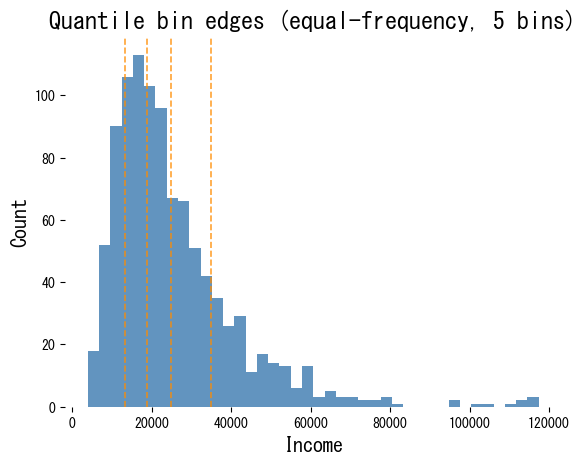
- Equal-frequency (quantile) binning divides the sorted data so that each bin has approximately the same number of observations (
pandas.qcut).
Equal-frequency bins are more robust to heavy tails, whereas equal-width bins preserve the notion of distance.
Visualising quantile bins #
| |
Comparing qcut and cut
#
| |
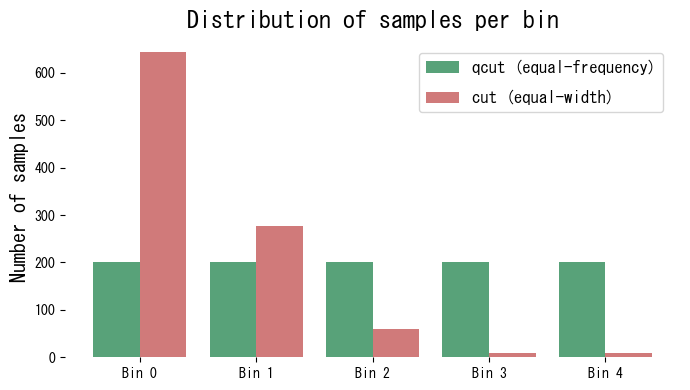
Equal-frequency binning produces almost identical counts for each bin, while equal-width binning assigns many observations to the dense centre and few to the extremes.
Practical tips #
- Clip extreme outliers before binning; even a single extreme value can stretch the range and break equal-width bins.
- Store the edges produced during training and reuse them later to ensure identical bin definitions.
- Tree-based models rarely need explicit binning. For linear models, however, binning can capture non-linear effects while keeping the feature space compact.