Yeo-Johnson transformation

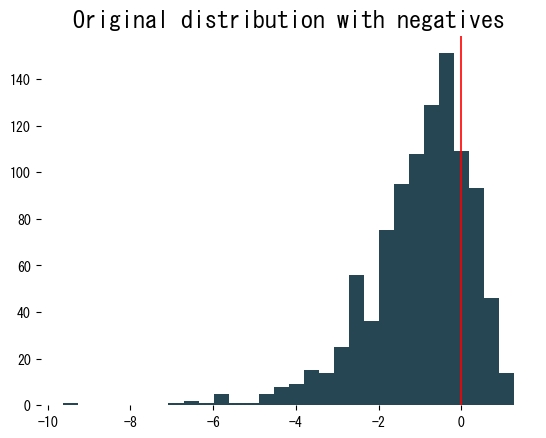
Last updated 2025-11-03 Read time 2 min

<p>The <b>Yeo-Johnson</b> power transformation is a Box-Cox style transform that can stabilise variance and make skewed numerical features look more Gaussian <em>even when the data contain zeros or negative values</em>.</p>

scipy.stats.yeojohnson

Definition #

For an observation (y) and power parameter (\lambda), the Yeo-Johnson transform (T_\lambda(y)) is defined piecewise:

$$ T_\lambda(y)= \begin{cases} \dfrac{(y + 1)^\lambda - 1}{\lambda}, & y \ge 0,\ \lambda \ne 0,\\\\ \log(y + 1), & y \ge 0,\ \lambda = 0,\\\\ -\dfrac{(1 - y)^{2 - \lambda} - 1}{2 - \lambda}, & y < 0,\ \lambda \ne 2,\\\\ -\log(1 - y), & y < 0,\ \lambda = 2. \end{cases} $$

When (\lambda = 1) the transform leaves the data unchanged.
Positive observations are treated like a Box-Cox transform on (y + 1).
Negative observations are reflected around zero, allowing the method to cope with sign changes.
The inverse transform is defined by solving the same cases for (y); SciPy provides it via scipy.stats.yeojohnson_inverse.

The parameter (\lambda) is usually estimated by maximising the log-likelihood of the transformed data under a normal model. SciPy exposes the maximum-likelihood estimate through yeojohnson_normmax.

I. Yeo and R.A. Johnson, “A New Family of Power Transformations to Improve Normality or Symmetry”, Biometrika 87(4), 2000.

Worked example #

1
2
3
4
5
6
7
8
from scipy import stats
import matplotlib.pyplot as plt

x = stats.loggamma.rvs(1, size=1_000) - 0.5
plt.hist(x, bins=30)
plt.axvline(x=0, color="r")
plt.title("Original distribution with negatives")
plt.show()

Worked example figure

1
2
3
4
5
6
7
8
9
from scipy.stats import yeojohnson, yeojohnson_normmax

lmbda = yeojohnson_normmax(x)  # maximum-likelihood estimate of λ
print(f"Estimated λ: {lmbda:.3f}")

x_trans = yeojohnson(x, lmbda=lmbda)
plt.hist(x_trans, bins=30)
plt.title("After Yeo-Johnson")
plt.show()

Worked example figure

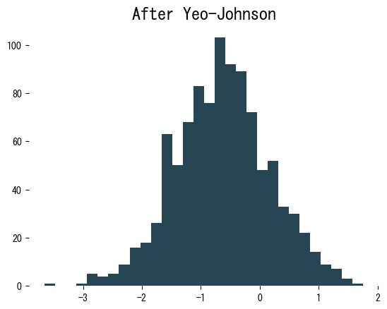
The histogram after transformation is much closer to symmetric. Because we explicitly pass lmbda, we can reuse the same parameter for validation or test data:

1
2
X_train_trans = yeojohnson(X_train, lmbda=lmbda)
X_valid_trans = yeojohnson(X_valid, lmbda=lmbda)  # reuse training λ

Practical tips #

Standardise features after the power transform if your model expects zero mean and unit variance.
Apply the transformation parameters learned on the training split to every other split to avoid data leakage.
When heavy tails remain, compare Yeo-Johnson with robust scalers such as RobustScaler; combining them often works well.

This transformation is a drop-in replacement for Box-Cox in preprocessing pipelines that cannot assume strictly positive data.