1
2
3
4
5
6
7
8
9
10
11
12
13
14
15
16
17
18
19
20
21
22
23
24
25
26
27
28
29
30
31
32
33
34
35
36
37
38
39
40
41
42
43
44
45
46
47
48
49
50
51
52
53
54
55
56
57
58
59
60
61
62
63
64
65
66
67
68
69
70
71
72
73
74
75
76
77
78
79
80
81
82
83
84
85
86
87
88
89
90
91
92
93
94
95
96
97
98
99
100
101
102
103
104
105
106
107
108
109
110
111
112
113
114
115
116
117
118
119
120
121
122
123
124
125
126
127
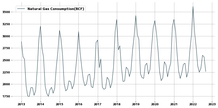
| data = {
"value": {
"2013-01-01": 2878.8,
"2013-02-01": 2567.2,
"2013-03-01": 2521.1,
"2013-04-01": 1967.5,
"2013-05-01": 1752.5,
"2013-06-01": 1742.9,
"2013-07-01": 1926.3,
"2013-08-01": 1927.4,
"2013-09-01": 1767.0,
"2013-10-01": 1866.8,
"2013-11-01": 2316.9,
"2013-12-01": 2920.8,
"2014-01-01": 3204.1,
"2014-02-01": 2741.2,
"2014-03-01": 2557.9,
"2014-04-01": 1961.7,
"2014-05-01": 1810.2,
"2014-06-01": 1745.4,
"2014-07-01": 1881.0,
"2014-08-01": 1933.1,
"2014-09-01": 1809.3,
"2014-10-01": 1912.8,
"2014-11-01": 2357.5,
"2014-12-01": 2679.2,
"2015-01-01": 3115.0,
"2015-02-01": 2925.2,
"2015-03-01": 2591.3,
"2015-04-01": 2007.9,
"2015-05-01": 1858.2,
"2015-06-01": 1899.9,
"2015-07-01": 2067.7,
"2015-08-01": 2052.7,
"2015-09-01": 1901.3,
"2015-10-01": 1987.3,
"2015-11-01": 2249.1,
"2015-12-01": 2588.2,
"2016-01-01": 3091.7,
"2016-02-01": 2652.3,
"2016-03-01": 2356.3,
"2016-04-01": 2083.9,
"2016-05-01": 1965.8,
"2016-06-01": 2000.7,
"2016-07-01": 2186.6,
"2016-08-01": 2208.4,
"2016-09-01": 1947.8,
"2016-10-01": 1925.2,
"2016-11-01": 2159.5,
"2016-12-01": 2866.3,
"2017-01-01": 2913.8,
"2017-02-01": 2340.2,
"2017-03-01": 2523.3,
"2017-04-01": 1932.0,
"2017-05-01": 1892.0,
"2017-06-01": 1910.4,
"2017-07-01": 2141.6,
"2017-08-01": 2093.8,
"2017-09-01": 1920.5,
"2017-10-01": 2031.5,
"2017-11-01": 2357.3,
"2017-12-01": 3086.0,
"2018-01-01": 3340.9,
"2018-02-01": 2710.7,
"2018-03-01": 2796.7,
"2018-04-01": 2350.5,
"2018-05-01": 2055.0,
"2018-06-01": 2063.1,
"2018-07-01": 2350.7,
"2018-08-01": 2313.8,
"2018-09-01": 2156.1,
"2018-10-01": 2285.9,
"2018-11-01": 2715.9,
"2018-12-01": 2999.5,
"2019-01-01": 3424.3,
"2019-02-01": 3019.1,
"2019-03-01": 2927.8,
"2019-04-01": 2212.4,
"2019-05-01": 2134.0,
"2019-06-01": 2119.3,
"2019-07-01": 2393.9,
"2019-08-01": 2433.9,
"2019-09-01": 2206.3,
"2019-10-01": 2306.5,
"2019-11-01": 2783.8,
"2019-12-01": 3170.7,
"2020-01-01": 3320.6,
"2020-02-01": 3058.5,
"2020-03-01": 2722.0,
"2020-04-01": 2256.9,
"2020-05-01": 2072.2,
"2020-06-01": 2127.9,
"2020-07-01": 2464.1,
"2020-08-01": 2399.5,
"2020-09-01": 2151.2,
"2020-10-01": 2315.9,
"2020-11-01": 2442.0,
"2020-12-01": 3182.8,
"2021-01-01": 3343.9,
"2021-02-01": 3099.2,
"2021-03-01": 2649.4,
"2021-04-01": 2265.1,
"2021-05-01": 2117.4,
"2021-06-01": 2238.4,
"2021-07-01": 2412.2,
"2021-08-01": 2433.8,
"2021-09-01": 2142.3,
"2021-10-01": 2262.6,
"2021-11-01": 2693.3,
"2021-12-01": 3007.3,
"2022-01-01": 3612.1,
"2022-02-01": 3064.2,
"2022-03-01": 2785.4,
"2022-04-01": 2379.3,
"2022-05-01": 2247.8,
"2022-06-01": 2326.9,
"2022-07-01": 2597.9,
"2022-08-01": 2566.1,
"2022-09-01": 2263.3,
}
}
data = pd.DataFrame(data)
data.rename(columns={"value": "Natural Gas Consumption(BCF)"}, inplace=True)
data.index = pd.to_datetime(data.index)
data = data.asfreq("MS")
data.head()
|